Sampling phonon spectra from molecular-dynamics simulations

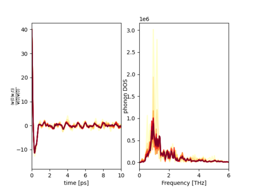
Phonon spectra can be obtained as the power spectrum of the normalized velocity-autocorrelation function [1][2]. The velocities of the ions and hence the velocity-autocorrelation function are recorded during a molecular dynamics (MD) simulation. Fig. 1 shows the example of CsPbBr$_3$ which is discussed in more detail below.
In contrast to the phonon DOS computed by Fourier interpolation of the force-constant matrix, analyzing the power spectrum does not rely on mapping to a model Hamiltonian. It naturally accounts for anharmonic contributions, as well as temperature dependence.
Phonon spectra step-by-setp
For the setup of the MD simulation and choice of ensemble, two aspects need to be taken into account:
- To have a well-defined reciprocal space, the simulation has to be done at constant volume.
- To probe the velocity-autocorrelation function, no thermostat should interfere with the recorded velocities.
Hence, the following describes how to compute the phonon spectra by sampling an NVE ensemble starting from thermalized structures.
Step 1: Generate thermalized initial structures
Run an NVT simulation using the Langevin thermostat to generate thermalized initial structures. The choice of thermostat is crucial. The Langevin thermostat is well-suited because it is a stochastic thermostat and populates all available phonon modes of our system uniformly, as white noise is added to the velocity autocorrelation due to random forces in each time step. The size of the system must be chosen such that the dimensions of the supercell are large enough to accommodate the phonon modes. Ideally, the time step (POTIM) is chosen such that the frequency of the fastest phonon mode of interest can still be resolved. Run the NVT simulation until the system is thermalized. Then, sample approximately 10 structures from the MD trajectory with a spacing of one or two times the self-correlation time and store the initial structures as POSCAR files.
Step 2: Sample velocities from NVE simulations for each initial structure
For each initial structure, perform an NVE simulation with VELOCITY = True . The minimum simulation time requires roughly two slowest phonon cycles, which is dictated by the decay time of a preliminary trajectory's normalized velocity autocorrelation function to zero. The velocities are written to vaspout.h5 and can be accessed using py4vasp with
import py4vasp as pv
calc = pv.Calculation.from_path("path/to/calc")
velocity_dict = calc.velocity[:].read()
Step 3: Compute normalized velocity autocorrelation function for each NVE simulation
The normalized velocity autocorrelation function for an $N$-particle system is given by \begin{equation} f(t)=\sum_{s=1}^{types}f_{s}(t)=\frac{\langle \sum_{s=1}^{types}\sum_{i=1}^{N_{s}}\mathbf{v}_{i}(\Delta T)\mathbf{v}_{i}(\Delta T+t) \rangle}{\mathbf{v}_{i}(\Delta T)\mathbf{v}_{i}(\Delta T)}. \end{equation} The brackets $\langle ,\rangle$ denote a thermal average which has to be computed over different MD trajectories and starting times $\Delta T$ within each trajectory. The sum over $i$ runs over the atoms within each species, and the sum $s$ is over all atomic species contained in the simulated system.
Step 4: Compute the power spectrum for each normalized velocity autocorrelation function
The phonon spectral function is the power spectrum of $f_{s}(t)$ and is obtained by performing the following Fourier transformation: \begin{equation} g(\omega)=\sum_{s=1}^{types}g_{s}(\omega)=\left| \sum_{s=1}^{types}\int_{-\infty}^{\infty}f_{s}(t)e^{-i\omega t}\right|^{2}. \end{equation}
Step 5: Compute averages and check for convergence
To check for convergence, $f(t)$ and $g(\omega)$ obtained for each NVE trajectory can be successively averaged. To this end, plot a single trajectory, compared to an average over 2 trajectories, and so on. If needed, the above steps can be repeated to generate additional data to reach the desired accuracy.
| Tip: For further information on phonon signal analysis Ref[2] might be a helpful source. |
Example
Setup and auxilary scripts
First, create thermalized initial structures. A simple INCAR file, which will perform an NVT simulation could look as follows
# INCAR molecular-dynamics tags NVE ensemble
IBRION = 0                   # choose molecular-dynamics
ISIF = 0                     # save time. No stress tensor. Box shape fixed.
MDALGO = 3                   # using Langevin thermostat
TEBEG = 500                  # set temperature
LANGEVIN_GAMMA = 0.5 0.5 0.5 # Langevin friction coefficient for 3 atomic species
NSW = 10000                  # number of time steps
POTIM = 2.0                  # time step in femto seconds
A bash script to produce 10 starting configurations in the form of POSCAR files could look as follows
# Equilibrate.sh script to generate POSCAR_1 to POSCAR_10
for i in {1..10}; do
   cp POSCAR POSCAR_$i
   mpirun -np 32 vasp_std
   cp CONTCAR CONTCAR_$i
   cp CONTCAR POSCAR
done
This bash script will create POSCAR_i where $i$ runs from 1 to 10. These serve as initial structures including inital velocities for the NVE simulations.
Secondly, sample velocities from NVE simulations for each initial structure. An INCAR file can look as follows:
# INCAR molecular-dynamics tags NVE ensemble
IBRION = 0                   # choose molecular-dynamics
ISIF = 0                     # save time. No stress tensor. Box shape fixed.
MDALGO = 1                   # using Andersen thermostat
ANDERSEN_PROB = 0.0          # setting Andersen collision probability to zero to get NVE ensemble
TEBEG = 500                  # set temperature
NSW = 10000                  # number of time steps
POTIM = 2.0                  # time step in femto seconds
VELOCITY = T                 # make sure to write velocities to vaspout.h5
Again, it is advisable to use a script to generate NVE trajectories. The following bash script will assume a base folder containing POSCAR files named POSCAR_1 to POSCAR_10, an INCAR file, a KPOINTS file and an POTCAR file. The script will create folders Run1 to Run10. Each folder will contain a vaspout.h5 file after script execution. These vaspout.h5 files will be needed for the analysis scripts of the next section.
# Run NVE MD simulation for each inital configuration
for i in {1..10}; do
   mkdir Run$i
   cd Run$i
   cp ../INCAR .
   cp ../KPOINTS .
   cp ../POSCAR_${i} POSCAR
   vasp_std
   cd ..
done
The following Python script can be used to compute normalized velocity-autocorrelation functions
import numpy as np
class AutoCorrelation:
    """
    A class to compute the velocity auto-correlation function for a given set of velocity data.

    Attributes:
    -----------
    delta : int, optional
        The step size for time intervals in the computation (default is 1).

    Methods:
    --------
    velocity_auto_correlation(velos):
        Computes the velocity auto-correlation function for the input velocity data.
    """
    def __init__( self, delta = 1 ):
        """
        Initializes the AutoCorrelation object with a specified time step size.

        Parameters:
        -----------
        delta : int, optional
            The step size for time intervals in the computation (default is 1).
        """
        self.delta = delta
    def velocity_auto_correlation( self, velos ):
        """
        Computes the velocity auto-correlation function for the given velocity data.

        Parameters:
        -----------
        velos : numpy.ndarray
            A 3D array of shape (Nt, Nx, Ndim) representing the velocity data, where:
            - Nt is the number of time steps,
            - Nx is the number of particles,
            - Ndim is the number of spatial dimensions.

        Returns:
        --------
        numpy.ndarray
            A 2D array of shape (Nt // 2, Nx) representing the velocity auto-correlation function
            for each particle over time.

        Notes:
        ------
        - The function normalizes the correlation values using the squared norm of the initial velocities.
        - The computation is performed for time intervals up to Nt // 2.
        """
        Nt, Nx, Ndim = velos.shape
        deltaT = self.delta
        corr_func = np.zeros( [ Nt // 2, Nx ] )
        counter   = np.zeros( [ Nt // 2, 1 ] )
        for dt in range( 0, Nt//2, deltaT ):
            v0   = velos[ dt, :, : ]
            norm = np.asarray( [ np.linalg.norm( v0[ i, : ] )**2 for i in range( Nx ) ] )
            for t in range( dt, Nt//2 ):
                vt = velos[ t, :, : ]
                value = np.asarray( [ np.dot( vt[i,:], v0[ i, : ] ) for i in range( Nx ) ] )
                corr_func[ t-dt, : ] += value / norm
                counter[ t-dt ] += 1
        return corr_func / counter
The following python script can be used to obtain the phonon density of states by computing the power spectra of the normalized velocity auto correlation functions.
import sys
import py4vasp
import numpy as np
import matplotlib.pyplot as plt


import ComputeCorrelation

class ComputePhonons:
    """
    @brief Class to compute phonon-related properties such as autocorrelation, power spectra, and averages.

    This class provides methods to compute velocity autocorrelation, power spectra, and averages for atomic systems
    based on velocity data. It also includes functionality to write the computed data to files.

    @class ComputePhonons
    """
    def __init__( self, fname, dt = 1.0, timeShift=50 ):
        """
        @brief Constructor to initialize the ComputePhonons object.
        @param fname Path to the input file for the calculation.
        @param dt Time step in femtoseconds (default: 1.0).
        @param timeShift Time shift for autocorrelation computation (default: 50).
        """
        self.fname  =  fname
        self.calc   =  py4vasp.Calculation.from_path( self.fname )
        self.velos  =  self.calc.velocity[:].read()
        self.time_step =  dt /1000 # thz output
        self.timeShift = timeShift

    def compute_ac( self ):
        """
        @brief Compute the velocity autocorrelation function.
        This method calculates the velocity autocorrelation function using the provided velocity data.
        """
        dos     =  ComputeCorrelation.AutoCorrelation( self.timeShift )
        self.ac =  dos.velocity_auto_correlation( self.velos["velocities"] )

    def compute_averages( self ):
        """
        @brief Compute averages of the autocorrelation function for total and per-atom contributions.
        This method calculates the total autocorrelation and groups the autocorrelation by atomic species.
        """
        unique, counts = np.unique_counts( self.velos["structure"]["elements"] )
        self.total_ac = np.sum( self.ac, axis=1 )
        labels = self.velos["structure"]["elements"]
        unique_labels, inverse = np.unique(labels, return_inverse=True)
        result = np.zeros((self.ac.shape[0], len(unique_labels)), dtype=self.ac.dtype)
        np.add.at(result, (slice(None), inverse), self.ac )
        self.atom_ac = {label: result[:, i] for i, label in enumerate(unique_labels)}

    def compute_power_spectra( self ):
        """
        @brief Compute the power spectra for total and per-atom contributions.
        This method calculates the power spectra using the Fourier transform of the autocorrelation functions.
        """
        self.ps_total = np.abs( np.fft.fft( self.total_ac ) )**2
        self.ps_atom  = {}
        for key in self.atom_ac.keys():
            self.ps_atom[key] = np.abs( np.fft.fft( self.atom_ac[key] ) )**2

        freqs = np.fft.fftfreq( self.ps_total.shape[0], self.time_step )
        self.ps_total = np.vstack( [freqs, self.ps_total/np.max(self.ps_total)] ).T
        self.ps_total = self.ps_total[ :self.ps_total.shape[0]//2, : ]
        for key in self.ps_atom.keys():
            self.ps_atom[key] = np.vstack( [freqs, self.ps_atom[key]/np.max( self.ps_atom[key] )] ).T
            self.ps_atom[key] = self.ps_atom[key][ :self.ps_atom[key].shape[0]//2, : ]

    def write_total_ps( self, fname="total_ps.dat" ):
        """
        @brief Write the total power spectrum to a file.
        @param fname Name of the output file (default: "total_ps.dat").
        """
        np.savetxt( fname, self.ps_total )

    def write_total_ac( self, fname="total_ac.dat" ):
        """
        @brief Write the total autocorrelation function to a file.
        @param fname Name of the output file (default: "total_ac.dat").
        """
        x = np.linspace( 0, self.time_step*self.total_ac.shape[0], self.total_ac.shape[0] )
        result = np.vstack( [x, self.total_ac] ).T
        np.savetxt( fname, result )

    def write_atom_ac( self ):
        """
        @brief Write the per-atom autocorrelation functions to files.
        Each atomic species' autocorrelation function is written to a separate file.
        """
        for key in self.ps_atom.keys():
            np.savetxt( f"{key}_ps.dat", self.ps_atom[key] )

     def write_atom_ps( self ):
         """
         @brief Write the per-atom power spectra to files.
         Each atomic species' power spectrum is written to a separate file.
         """
         for key in self.ps_atom.keys():
             np.savetxt( f"{key}_ps.dat", self.ps_atom[key] )


 if __name__=="__main__":
     x = ComputePhonons( sys.argv[1], float(sys.argv[2]) )
     x.compute_ac()
     x.compute_averages()
     x.compute_power_spectra()
     x.write_total_ps()
     x.write_total_ac()
     x.write_atom_ps()
     x.write_atom_ac()
The PhononDOS.py script can be used to compute the phonon spectral function for a given NVE simulation folder containing an vaspout.h5 file created with the aforementioned INCAR file. The script will create a file called total_ps.dat containing the total phonon spectral function. The partial phonon spectra of the atomic species are written to files ElementKey_ps.dat. As input, the script needs a folder name containing a vaspout.h5 file, and the second input argument has to be the simulation time step of your simulation in fs. The written files will contain the frequency in THz as the first column. The second column will contain the phonon spectra computed as the power spectrum of the velocity autocorrelation function.
Anharmonic ratteling in CsPbBr$_{3}$

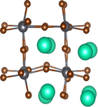
In the following the convergence of the phonon DOS will be exemplified on the CsPbBr$_{3}$ in the cubic phase at 500K. A snapshot of the used simulation box is shown in Fig. 2. The CsPbBr$_{3}$ consists of a cubic lead bromide framework which is covalently bonded. The cavities formed by the cubic lead-bromide framework are filled with weakly bonded Cs$^{+}$ cations. This makes the CsPbBr$_{3}$ a good example to test methods for anharmonic phonons.
The convergence of the phonon spectral function of CsPbrBr$_{3}$ is visualized in a single plot shown in Fig. 1. The yellow line shows an average over a single trajectory. The more red the lines are, the more trajectories have been used for computing the average. The dark red line shows the average computed over all 10 trajectories. Based on the plot in Fig. 1, it is possible to conclude that enough data was obtained to properly converge the phonon spectral function.
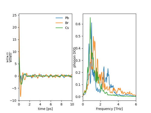
Fig. 3 shows the atom-resolved normalized autocorrelations and phonon spectra. A peak in the Cs$^{+}$ cation phonon spectral function is visible around 1THz. This peak can be assigned to Cs$^{+}$ rattling frequencies coupling to optical phonon modes formed by the oscillations of the lead bromide framework.
For further information it is advised to take a look at Ref[2] or Ref[3] in which Cs$^{+}$ rattling modes were tuned to adjust the thermal conductivity of the material.

References
Related tags and articles
Molecular-dynamics calculations,
