Part 2: DFT+U and DFT+DMFT ¶

This notebook follows the workshop folder structure in this repository. You will run VASP (DFT and DFT+U) and then perform DFT+DMFT with solid_dmft (TRIQS, see instructions for installation and install_triqs.txt for installing on your local machine) using the projectors from VASP (PLOs).

Content¶

 4 DFT in paramagnetic and antiferromagnetic: preparing for DMFT
 5 Antiferromagnetic DFT+U and DOS
 6 DFT+DMFT one-shot (Hartree)
 7 DFT+DMFT charge self-consistent (Hartree)
 8 Comparing antiferromagnetic to paramagnetic and Hartree to QMC

4 DFT SCF calculation and preparing for DMFT

$\uparrow$

¶

By the end of this section, you will be able to:

• Set up and run DFT calculations for antiferromagnetic unit cell of NiO.
• Control the generation of Ni-d projectors needed for DMFT (Dynamical Mean-Field Theory).
• Learn about relevant output files from VASP for DMFT calculations
• Extract the $U$ and $J$ values from a cRPA (constrained random-phase approximation) calculation required for running DMFT calculations.

4.1 Task¶

Perform a non-magnetic (NM) DFT calculation for the antiferromagnetic (AFM) unit cell of NiO, generating input for dynamical mean-field theory (DMFT): local orbitals converted to projected local orbitals (PLOs), and extracting the U and J value from a previous cRPA calculation

DFT+U is a computationally inexpensive correction to standard DFT designed to better describe strongly correlated electrons in localized orbitals (typically $d$ or $f$ shells). Standard (semi-)local exchange-correlation functionals suffer from spurious self-interaction, artificially delocalizing electrons and underestimating band gaps in Mott insulators and correlated metals. DFT+U remedies this in a very simple yet successful way by adding a Hubbard-like on-site Coulomb penalty $U$ for double occupation of the target subspace. In the simplified rotationally invariant form by Dudarev et al. [Phys. Rev. B 57 (1998) 1505], the total energy reads:

$$\tag{4.1} E=E_{DFT}+\sum_I\left[\frac{U^I}{2} \sum_{m, \sigma \neq m^{\prime}, \sigma^{\prime}} n_m^{I \sigma} n_{m^{\prime}}^{I \sigma^{\prime}}-\frac{U^I}{2} n^I\left(n^I-1\right)\right] $$

where $n_m^{I \sigma}$ is the occupation of orbital $m$ with spin $\sigma$ on site $I$. The second term, $\frac{U^I}{2} n^I\left(n^I-1\right)$ is the so-called double counting correction, which subtracts an estimate of the interaction energy already included in $E_\mathrm{DFT}$, preventing it from being counted twice.

The bracketed term vanishes for integer occupations, leaving $E_\mathrm{DFT}$ unchanged in the atomic limit, but penalizes fractional occupations and drives the system toward more localized, integer-like solutions. While DFT+$U$ is cheap and often qualitatively correct, the parameter $U$ must be chosen carefully (e.g., via cRPA or linear-response - see below), and the method cannot capture dynamical correlation effects or Kondo physics — motivating the use of DFT+DMFT for more demanding cases.

In this exercise, you will do a non-spin-polarized DFT calculation on antiferromagnetic (AFM) NiO, preparing local orbitals and extract $U$ and $J$ values for DFT+$U$ in subsequent calculations.

4.2 Input¶

The input files to run the DFT ground state calculation are prepared at $TUTORIALS/strongly_correlated/e04_scf. Check them out!

POSCAR:

AFM NiO
4.171
1.0 0.5 0.5
 0.5 1.0 0.5
 0.5 0.5 1.0
 2 2
Cartesian
 0.0 0.0 0.0
 1.0 1.0 1.0
 0.5 0.5 0.5
 1.5 1.5 1.5

INCAR:

A DFT run. We have tightened EDIFF, and increased NELMIN and NBANDS to ensure tight convergence. Below, we emphasize some of the tags specific to this type of calculation:

• System names the system.
• NCORE controls how many cores work on the FFTs (fast Fourier transform) of each band.
• KPAR controls how many $\textbf{k}$-points are treated in parallel.
• ISMEAR sets smearing parameter, in this case the Tetrahedron method with Blöchl corrections without smearing.
• KSPACING generates a $\textbf{k}$-mesh with a spacing of that value between the $\textbf{k}$-points.
• EDIFF defines the electronic break condition. This is very tight to ensure tight convergence of the wavefunction and KS eigenvalues (cf. norm of the residual rms in OSZICAR).
• NELMIN specifies the minimum number of electronic self-consistency steps.
• NBANDS specifies the number of Kohn-Sham orbitals.
• LORBIT selects a projection method of the orbitals onto the atomic sphere.
• EMIN sets the lower boundary energy limit for evaluating the density of states (DOS).
• EMAX sets the upper boundary energy limit for evaluating the density of states (DOS).
• NEDOS sets the number of grid points for the DOS.
• LMAXMIX defines the l-quantum number up to which the one-center PAW charge densities are passed through the charge density mixer and written to the CHGCAR.
• LOCPROJ specifies local functions on which the orbitals are projected.

System  = AFM NiO

NCORE = 1
KPAR = 4

ISMEAR = -5
SIGMA = 0.1

KSPACING = 0.4

# converge wave functions
EDIFF = 1.E-10
NELMIN = 35
NBANDS = 32

# the energy window to optimize projector channels (absolute)
LORBIT = 14
EMIN = -6
EMAX = 18
NEDOS = 5001

LMAXMIX = 4

# project to Ni d 
LOCPROJ = "1 2 : d : Pr"

KPOINTS:

Defined using KSPACING in the INCAR

POTCAR:

Here we use the Ni_pv to treat the important $p$ valence states explicitly, which weakly hybridize with the $d$-orbitals. This can strongly impact the band structure and lattice parameter, so it is important to choose the right pseudopotential. Ideally, we would use the Ni_sv_GW potentials, but do not for the sake of time.

   PAW_PBE Ni_pv 06Sep2000
   PAW_PBE O 08Apr2002      

4.3 DFT calculation¶

Open a terminal, navigate to this example's directory and run VASP by entering the following:

cd $TUTORIALS/strongly_correlated/e04_scf/
mpirun -np 4 vasp_std

This performs a standard density functional theory (DFT) calculation, specifically a non-magnetic (NM) calculation.

Let's take a look at a few of the key INCAR tags. We specify the projectors to be created via the LOCPROJ tag for the Ni-$d$ orbitals. Additionally, we specify the LORBIT tag to 14 to optimize the projectors in the given energy range EMIN to EMAX. Projecting on the PAW projectors leaves us with a choice to which PAW projector channel the projection is done. With this tag we automatically optimize the projector channel choice in this specific energy window. The number of bands is slightly increased and the convergence criteria are stricter to converge the KS wavefunction (RMS).

The end of the std out should look like this for the smaller unit cell:

    DAV:  34    -0.113735946306E+02   -0.11278E-09    0.18183E-14  1208   0.167E-10    0.675E-04
    DAV:  35    -0.113735946308E+02   -0.14415E-09   -0.80060E-13  1232   0.948E-11    0.675E-04
    DAV:  36    -0.113735946307E+02    0.42746E-10   -0.66442E-13  1224   0.176E-10
     LOCPROJ mode
     Computing AMN (projections onto localized orbitals)
       1 F= -.11373595E+02 E0= -.11368913E+02  d E =-.936338E-02
     writing wavefunctions

Once the calculation is finished, take a look at the structure using py4vasp:

After this, you should have at least the vaspout.h5, and the projector output (LOCPROJ/PROJCAR) in the directory e04_scf. From this calculation we will then construct the DMFT (dynamical mean-field theory) input for TRIQS/solid_dmft.

4.4 PLO construction and conversion¶

4.4.1 Task¶

In DFT+DMFT, we need a correlated subspace (here: Ni $3d$). In this tutorial, we use projected local orbitals (PLOs). PLOs are constructed in VASP in the same way it is done for the LDAU tag by projecting the KS (Kohn-Sham) states $| \tilde{\Psi}_{\nu \mathbf{k}} \rangle$ on localized orbitals provided by the PAW formalism:

$$\tag{4.2} P^{\mathbf{R}}_{L,\nu}(\mathbf{k}) = \sum_i \langle \chi^{\mathbf{R}}_L | \phi_i \rangle \langle \tilde{p}_i | \tilde{\Psi}_{\nu \mathbf{k}} \rangle,$$

where $|\chi^{\mathbf{R}}_L\rangle$ are localized basis functions associated with each correlated site R, $|\phi_i \rangle$ are all-electron partial waves, and $| \tilde{p}_i\rangle$ are the standard PAW projectors. $L$ is a compound index of local quantum numbers. The raw projectors are orthonormalized and connect the KS basis $\nu$ with the localized orbitals $m$: $P^{\mathbf{R}}_{m,\nu}(\mathbf{k})$ at $k$-point $\mathbf{k}$.

These local projections are selected by LOCPROJ and written to the LOCPROJ (which will be converted to the PLOs) and PROJCAR files (which contain the information in human-readable format). We will use TRIQS/dft_tools to process these raw projectors. plo.cfg defines which shells (orbitals + ions) are used as correlated orbitals and which KS bands/energy window are/is projected, see also plo converter documentation for detailed information. The converter.py TRIQS/dft_tools reads the VASP output and creates vasp.h5 (DFT+DMFT input for TRIQS/solid_dmft).

4.4.2 Conversion¶

Let's have a look at the plo.cfg file, which sets up the information for converting the local projections to PLOs for TRIQS / DMFT:

The key entries for us in plo.cfg are:

• EWINDOW: energy window used for finding the relevant KS states
• BANDS: band index window (VASP band indices) used for the projection (the raw projectors in VASP are done for all bands).
• LSHELL = 2: $d$-shell
• IONS: which atoms carry the correlated $d$-shell (antiferromagnetic: two Ni)
• CORR = True: marks this shell as correlated (i.e. treated by DMFT)

Navigate to the e04_scf/ and run the conversion:

cd $TUTORIALS/strongly_correlated/e04_scf/
python ../scripts/converter.py &> log.converter

This produces (among others) the vasp.h5 file and also DOS for the projector functions in pdos_*.dat from the PLO step. Have a look at log.converter with vi e04_*/log.converter. Once you have opened the file, navigate to the lines following Generating 1 shell.... You can also do this with:

grep -A 17 "Generating 1 shell..." $TUTORIALS/strongly_correlated/e04_scf/log.converter

  Generating 1 shell...
 
    Shell         : 1
    Orbital l     : 2
    Number of ions: 2
    Dimension     : 5
    Correlated    : True
    Ion sort      : [1, 2]
Density matrix:
  Shell 1
Site diag : True
    Site 1
     1.9562328    -0.0056879    -0.0014441    -0.0056863    -0.0000064
    -0.0056879     1.9562318     0.0007166    -0.0056853    -0.0012624
    -0.0014441     0.0007166     1.2855518     0.0007276    -0.0000328
    -0.0056863    -0.0056853     0.0007276     1.9562303     0.0012688
    -0.0000064    -0.0012624    -0.0000328     0.0012688     1.2854792
      trace:  8.439725912548175
    Site 2
     1.9562328    -0.0056879    -0.0014441    -0.0056863    -0.0000064
    -0.0056879     1.9562318     0.0007166    -0.0056853    -0.0012624
    -0.0014441     0.0007166     1.2855518     0.0007276    -0.0000328
    -0.0056863    -0.0056853     0.0007276     1.9562303     0.0012688
    -0.0000064    -0.0012624    -0.0000328     0.0012688     1.2854792
      trace:  8.43972591254552
 
  Impurity density: 16.879451825093696

NB your impurity density values may differ slightly.

Here, the output shows the generation of one impurity site for DMFT to be treated (same as in DFT+U, where one picks site+orbital). Note also the $(5 \times 5)$ occupation matrix generated via the PLOs: $n_m^{I \sigma}$.

Now let's compare the VASP projected DOS (from vaspout.h5) to the PLO-projected DOS (pdos_*.dat). This is a quick sanity check that your projector window captures the relevant Ni $d$-character.

The Ni $d$-states are shown in blue (VASP local projections) and cyan (PLOs). You can see how the local projections from VASP and the PLOs correspond well to one another, so that PLOs sufficiently capture the relevant Ni $d$-character require for our calculations.

NB there is a difference in the orthonormalization procedure between the local projection in VASP and TRIQS, hence the difference in height around -5 eV.

4.5 Extract U/J from cRPA (UIJKL_cRPA)¶

4.5.1 Task¶

In part 1, you calculated the screened Coulomb interaction of the Ni-$d$ shell. This information was stored in the UIJKL file. It contains the four-index, partially screened Coulomb interaction tensor (here at $\omega=0$):

$$\tag{4.3} \displaystyle{ U_{ijkl}^{\sigma\sigma'} = \int {\rm d}{\bf r}\int {\rm d}{\bf r}'w_{i}^{*\sigma}({\bf r}) w_{j}^{\sigma}({\bf r}) U({\bf r},{\bf r}',\omega) w_{k}^{*\sigma'}({\bf r}') w_{l}^{\sigma'}({\bf r}') } $$

where $w_{a}^{*\sigma}({\bf r})$ are the Wannier orbitals and $U({\bf r},{\bf r}',\omega)$ is the partially screened Coulomb potential.

You could use the UIJKL file from your previous calculations. In order to be closer to convergence, we have provided a file ($TUTORIALS/strongly_correlated/e04_scf/ref/UIJKL_cRPA_ref), which you will use for DFT+$U$ in the following exercise. You can also use the UIJKL file that you calculated in exercise e03, bearing in mind that you will get different results to those using UIJKL_cRPA).

4.5.2 Processing UIJKL¶

With the following python script, you will load the partially screened Coulomb interaction tensor. Then, the four-index tensor is fitted to a Slater-parameterized interaction Hamiltonian to extract effective Hubbard $U$ and Hund's coupling $J$ values for the Ni-$d$ shell. The resulting $U$ and $J$ values will be used in all subsequent DFT+$U$ and DFT+DMFT calculations:

If you would like to understand what is happening in more detail, see below:

The result is an effective Hubbard $U$ and Hund's coupling $J$ that best reproduce the original $U_{ijkl}$ within the Slater interaction form. For the rest of this tutorial we use the resulting ($U$,$J$) consistently in e05_dftu/INCAR and in the DMFT configs (e06_dmft_os/dmft_config.toml, e07_dmft_csc/dmft_config.toml, e08_dmft_os_qmc/dmft_config.toml).

In the next exercise, you will calculate the DFT+$U$ for AFM NiO using the parameters that you have generate in this exercise and part 1.

4.6 Questions¶

1. Which two VASP files contain the local projections?
2. Which TRIQS file contains the projected local orbitals?
3. What are projected local orbitals (PLOs) and how are they used to define a correlated subspace in DFT+DMFT?
4. What is screened Coulomb interaction, and how does it differ from the bare Coulomb interaction?

5 Antiferromagnetic DFT+U and DOS

$\uparrow$

¶

By the end of this section, you will be able to:

• Run an AFM DFT+U calculation with cRPA-derived interaction parameters.
• Analyse the spin-resolved DOS (density of states)
• Identify the insulating gap and the Ni-$d$ and O-$p$ orbital character.

5.1 Task¶

Calculate the DOS for AFM NiO using DFT+U (U=6.181 and J=1.134), then analyse the structure.

In this exercise, you will calculate and then analyse the bandgap for AFM NiO using DFT+U.

5.2 Input¶

The input files to run the DFT ground state calculation are prepared at $TUTORIALS/strongly_correlated/e05_dftu. Check them out!

POSCAR:

AFM NiO
4.171
1.0 0.5 0.5
 0.5 1.0 0.5
 0.5 0.5 1.0
Ni O
 2 2
Cartesian
 0.0 0.0 0.0
 1.0 1.0 1.0
 0.5 0.5 0.5
 1.5 1.5 1.5

INCAR:

A DFT run using DFT+U approach. Below, we emphasize some of the tags specific to this type of calculation:

• EFERMI defines how the Fermi energy is calculated; MIDGAP sets it to the middle of the bandgap.
• LASPH should be considered a standard setting, especially for magnetic calculations. It includes aspherical contribution to the gradient corrections inside the PAW spheres.
• ISPIN=2 turns on spin-polarization, enabling magnetic calculations.
• MAGMOM defines the initial magnetic moment for each atom.
• LDAU switches on the DFT+U method.
• LDAUTYPE=1 selects Liechtenstein's approach.
• LDAUL specifies the $l$-quantum number for which the on-site interaction is added.
• LDAUU sets the effective on-site Coulomb interactions $U$.
• LDAUJ Sets the effective on-site exchange interactions $J$.
• LDAUPRINT controls the verbosity of a DFT+U calculation.

System  = AFM NiO

NCORE = 1
KPAR = 4

ISMEAR = 0
SIGMA = 0.1
EFERMI = MIDGAP
KSPACING = 0.4

EDIFF = 1.E-8
NBANDS = 32

# the energy window to optimize projector channels (absolute)
LORBIT = 14
EMIN = -6
EMAX = 18
NEDOS = 5001

LMAXMIX = 4
LASPH = .TRUE.

ISPIN    = 2
MAGMOM   = 2.0 -2.0 2*0

LDAU      = .TRUE.
LDAUTYPE  = 1
LDAUL     = 2 -1
LDAUU     = 6.181 0.00
LDAUJ     = 1.134 0.00
LDAUPRINT = 1

KPOINTS:

Defined using KSPACING in the INCAR

POTCAR:

   PAW_PBE Ni_pv 06Sep2000
   PAW_PBE O 08Apr2002      

5.3 Calculation¶

Navigate to the e05_dftu/ directory and start the calculation with the following:

cd $TUTORIALS/strongly_correlated/e05_dftu
mpirun -np 4 vasp_std

The INCAR already contains LDAU* tags with $U$ and $J$ from cRPA:

    ISPIN    = 2
    MAGMOM   = 2.0 -2.0 2*0

    LDAU      = .TRUE.
    LDAUTYPE  = 1
    LDAUL     = 2 -1
    LDAUU     = 6.181 0.00
    LDAUJ     = 1.134 0.00

This will apply an extra Coulomb potential to the Ni $d$-shell and allow for magnetic ordering via ISPIN=2. For more information on magnetic ordering, see the tutorial Including on-site Coulomb interaction and pseudopotential selection for NiO relaxation.

A classic benchmark for DFT+$U$ is NiO, a prototypical Mott insulator with Ni in the $2+$ oxidation state ($d^8$). In an octahedral crystal field, the Ni $d$ orbitals split into a lower $t_{2g}$ triplet and an upper $e_g$ doublet. With 8 $d$ electrons, the $t_{2g}$ manifold is completely full (6 electrons, both spin channels), while the remaining 2 electrons occupy the $e_g$ manifold.

Once the calculation is finished, try plotting the DOS (density of states) for DFT (e04) and DFT+$U$ (e05):

The DOS from exercise e04 is shown as a dashed gray line. You can see now that there is a bandgap. We have opened this up using DFT+U (purple). The valence band maximum (VBM) and conduction band minimum (CBM) are shown in green. You can see that the bandgap is now slightly larger than 3 eV, creating an insulating gap. You can see that the total DOS (spin-up and spin-down) for the DFT+$U$ in the conduction band now has a large peak at ~2.5 eV, while the valence band has shifted to significantly lower energies.

So what happens when +$U$ is applied and magnetic ordering is allowed? Exchange splitting drives a high-spin $S=1$ configuration: the majority-spin $e_g$ states are fully occupied, and the minority-spin $e_g$ states are empty. DFT+$U$ pushes the occupied majority-spin $e_g$ states to lower energies and the empty minority-spin $e_g$ states to higher energies, opening a gap between them. Hence, we see a strong $e_g$ peak in the DOS at around 2.5 eV. The $t_{2g}$ shell, being completely full, is largely unaffected. The resulting gap is of charge-transfer character (O $2p$ → Ni $e_g$) rather than purely Mott–Hubbard, but DFT+$U$ nonetheless recovers a gap close to the experimental value of $\sim$4 eV [Phys. Rev. Lett. 53 (1984) 2339].

5.4 Questions¶

1. Which INCAR tags define the $U$ and $J$ parameters for DFT+$U$?
2. Why do we need to perform a spin-polarized DFT calculation, i.e., why does the gap not open when just applying DFT+$U$?
3. What does the large peak at 2.5 eV indicate?

6 DFT+DMFT one-shot (Hartree)

$\uparrow$

¶

By the end of this section, you will be able to:

• Set up and run a one-shot DFT+DMFT calculation using the static Hartree impurity solver via solid_dmft.
• Monitor and interpret DMFT convergence diagnostics from observables_*.dat and the h5 archive.
• Post-process the converged result to obtain the correlated spectral function and compare it to the DFT+U DOS.

6.1 Task¶

Calculate the DFT+DMFT@Hartree for AFM NiO and calculate the spectral function

While DFT focuses on self-consistent cycles to converge the energy and the electronic density, DFT+DMFT (dynamical mean-field theory) focuses on converging the Green's function and self-energy. The single-particle Green function $G(\mathbf{k}, \omega)$ is a central object in many-body theory, which encodes the probability amplitude for adding or removing an electron with momentum $\mathbf{k}$ and energy $\omega$ to the interacting system. It is the natural language for DMFT because it carries all the information needed to compute experimentally accessible observables: the spectral function $A(\mathbf{k},\omega) = -\frac{1}{\pi}\mathrm{Im}\, G(\mathbf{k},\omega+i0^+)$ is directly related to the intensity measured in angle-resolved photoemission spectroscopy (ARPES), and $\mathbf{k}$-integrated spectral function, which reduces to the non-interacting DOS when interactions are absent at 0 K, but in general carries additional information about quasiparticle lifetimes and Hubbard satellites accessible via (angle-integrated) photoemission.

To run these calculations, the key point to note is that the non-interacting Green's function is computed from the local projections (PLOs) and the KS eigenvalues $\epsilon_k$. From there, the $k$-integrated local Green's function $G_\mathrm{loc}$ in the PLO basis is calculated. Together with the local interaction Hamiltonian, these define the impurity problem within DMFT. Solving the impurity problem generates a new self-energy, which enters the Green's function and defines a self-consistency cycle. In this exercise, we will use an approximate impurity solver, which only evaluates the Hartree potential for the impurity problem.

Below, we go into more detail for those curious. On a first read-through, we recommend skipping over the theory and continuing with the exercise.

We have completed all preparations during the previous steps, and we are ready to run the one-shot DMFT calculation. Here we use the triqs/hartree_fock impurity solver (static self-energy). For density-density interactions, it should reproduce the physics of a DFT+$U$-like static mean-field and does not require any further parameters to set.

Since we have a limited amount of resources, we will only perform 5 DMFT iterations.

• Inspect the dmft_config.toml and verify that $U$, $J$, and the solver settings are correct.
• Run solid_dmft in e06_dmft_os/ and monitor convergence via observables_imp0_up.dat.
• Check that the chemical potential, impurity occupation, and self-consistency metrics converge.
• Run the post-processing script to obtain the Ni-$d$ spectral function and compare it to the DFT+$U$ DOS.

For the advanced theory, continue below; we recommend runnning e06 and e07 before reading through as those calculations take a long time:

The effect of interactions enters through the self-energy $\Sigma(\mathbf{k},\omega)$, which appears in the Dyson equation:

$$\tag{6.1} G(\mathbf{k},\omega)^{-1} = G_0(\mathbf{k},\omega)^{-1} - \Sigma(\mathbf{k},\omega), $$

where $G_0$ is the non-interacting Green's function. The real part of $\Sigma$ shifts and renormalizes quasiparticle energies, while the imaginary part gives their finite lifetime — both effects invisible to DFT+$U$ but naturally captured by DMFT.

DFT+$U$, used in the preceding step, can be understood as a static mean-field approximation to the Hubbard interaction: the self-energy is frequency-independent. DMFT generalizes this by retaining the full frequency dependence of the self-energy $\Sigma(\omega)$, thereby capturing dynamical correlation effects such as quasiparticle renormalization, Hubbard satellites, and the Kondo effect that are inaccessible to DFT+$U$. Formally, DMFT maps the lattice problem onto a single-site Anderson impurity model — a correlated impurity coupled to a self-consistently determined non-interacting bath — and the bath hybridization function encoded in the Weiss field $\mathcal{G}_0$ plays the role of the effective hopping between the impurity and its environment [Rev. Mod. Phys. 78 (2006) 865].

In one-shot DFT+DMFT (no charge self-consistency), DMFT is solved on top of a fixed DFT charge density [Rev. Mod. Phys. 78 (2006) 865]. The lattice self-energy is approximated by the impurity self-energy, and the self-consistency condition requires that the impurity Green's function $G_\mathrm{imp}$ equals the local ($\mathbf{k}$-summed) lattice Green's function $G_\mathrm{loc}$:

$$\tag{6.2} G_\mathrm{imp} = G_\mathrm{loc} $$

$G_\mathrm{loc}$ is obtained by summing the lattice Green's function over all $\mathbf{k}$-points, with the non-interacting dispersion $\epsilon_k$ (DFT eigenvalues) and the current impurity self-energy $\Sigma_\mathrm{imp}$:

$$\tag{6.3} G_\mathrm{loc} = \sum_k \frac{1}{i\omega_n + \mu - \epsilon_k - \Sigma_\mathrm{imp}} $$

Here $\mu$ is the chemical potential, adjusted at each iteration to enforce the correct total electron count (i.e., the impurity occupation $\sum_\sigma \langle n_\sigma \rangle$ matches the target filling). In practice the loop proceeds as follows: starting from an initial $\Sigma_\mathrm{imp}$ (typically zero), one computes $G_\mathrm{loc}$, then extracts the Weiss field — the bare Green's function of the effective bath — via Dyson's equation:

$$\tag{6.4} \left(\mathcal{G}_0^\mathrm{new}\right)^{-1} = \left(\sum_k \frac{1}{i\omega_n + \mu - \epsilon_k - \Sigma_\mathrm{imp}}\right)^{-1} + \Sigma_\mathrm{imp} $$

The Weiss field $\mathcal{G}_0$ fully encodes the bath: it tells the impurity solver how strongly and at what energies the correlated orbitals hybridize with the rest of the system. The impurity problem is then solved with this $\mathcal{G}_0$, yielding a new $\Sigma_\mathrm{imp}$, and the cycle repeats until convergence:

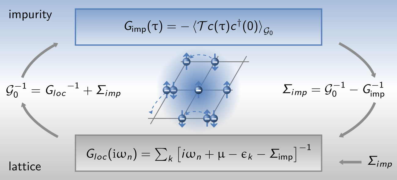
DFT+DMFT@Hartree denotes a further approximation in which the impurity solver is restricted to the Hartree level — the self-energy retains only its static (frequency-independent) Hartree contribution. This is computationally cheap and, for the purposes of this tutorial, serves as a sanity check connecting back to the DFT+$U$ result: a converged DFT+DMFT@Hartree solution should reproduce the DFT+$U$ DOS, since both correspond to a static mean-field treatment of the same interaction. The double counting correction should be placed inside of $\Sigma_\mathrm{imp}$ in the same way it is done for DFT+$U$.

6.2 Input¶

The input files to run the DFT+DMFT calculation are prepared at $TUTORIALS/strongly_correlated/e06_dmft_os. Check them out!

dmft_config.toml:
The program solid_dmft is controlled via a single configuration file.

The program solid_dmft is controlled via a single configuration file. This file is usually called dmft_config.toml but can be named differently when the name is passed as argument to solid_dmft. The file is divided into sections: general, solver, dft and advanced. It follows the typical toml file specification. Let's have a look at the config file we provide:

The most important parameters not yet introduced are U (similar to DFT+$U$), the choice of solver type of solver (Hartree in our case as introduced above), the number of DMFT iterations n_iter_dmft, the jobname where the calculation is performed in jobname, and the choice of double counting dc_type (similar to DFT+U). For now you can leave all parameters as is. Double check that the parameters $U$ and $J$ that we extracted above match the ones in the config file, cf. reference parameters.

While the calculation is running, you can inspect the progress with tail -f e06_dmft_os/out.

The calculation will create a directory beta20-hartree-afm, where everything will be stored in the h5 archive and text files. Take a look around and see if you can identify the important steps of a DMFT calculation (extracting local Green function, impurity solver, impurity occupations). Take special attention to the impurity density matrix printed before and after the solver runs. This is a good indicator of how well the calculation is going. Once convergence is reached, the input and output density matrices should be the same.

During the calculation, you can also monitor the observables_imp0_up.dat file (one file per impurity and per spin channel), which is stored in the jobname directory. This file summarizes the important observables in each iteration. Make sure that the chemical potential mu converges to a fixed value while the calculation is running.

 it |         mu |                                          G(beta/2) per orbital |                                                orbital occs up |   impurity occ up
  0 |    0.06631 |   -0.00421     -0.00421     -0.05537     -0.00421     -0.05537 |    0.97780      0.97780      0.64223      0.97780      0.64223 |           4.21787
  1 |    0.98725 |   -0.00016     -0.00016     -0.00034     -0.00016     -0.00034 |    0.98955      0.98955      0.97805      0.98955      0.97805 |           4.92473
  2 |    0.98725 |   -0.00000     -0.00000     -0.00000     -0.00000     -0.00000 |    0.99002      0.99003      0.98885      0.99002      0.98885 |           4.94777
  3 |    0.98725 |   -0.00000     -0.00000     -0.00000     -0.00000     -0.00000 |    0.99004      0.99004      0.98920      0.99004      0.98920 |           4.94852
  4 |    0.98725 |   -0.00000     -0.00000     -0.00000     -0.00000     -0.00000 |    0.99004      0.99004      0.98921      0.99004      0.98921 |           4.94855
  5 |    0.98725 |   -0.00000     -0.00000     -0.00000     -0.00000     -0.00000 |    0.99004      0.99004      0.98921      0.99004      0.98921 |           4.94855

Once the calculation has finished, we now plot the data and take a look at the most important observables to gauge if the calculation is converged:

• the chemical potential $\mu$ (mu)
• the impurity occupation per spin-channel (impurity occ up)
• the convergence of the Weiss field $\delta \mathcal{G}^0(i \omega_n)$
• the convergence of the DMFT self-consistency condition $\delta G_{imp}=|| G^{loc} - G^{imp} ||$

You can also check the convergence in conv_imp0.dat to find these metrics.

All metrics seem to indicate good convergence in the first few iterations. The last two plots show the most important metrics for DMFT calculation convergence: the Weiss field $\mathcal{G}^0(i \omega_n)$ and the convergence of DMFT self-consistency condition: $|| G^{loc} - G^{imp} ||$.

6.4 Post-processing - calculate the DOS and spectral function¶

The spectral function, which can be compared to photoemission (PES) experiments, is obtained by constructing first the lattice Green's functions $\hat G(k,\omega)$:

$$\tag{6.5} \hat G(k,\omega) = \left[ \omega + \mu -\hat{\epsilon}(k)-\left( \hat\Sigma(\omega)^{imp}-\hat\Sigma^{dc} \right) \right]^{-1} $$ where $\omega$ is the discrete Matsubara frequency, $\mu$ is the chemical potential, $\hat{\epsilon}(k)$ are the Kohn-Sham (KS) eigenvalues at $k$-point $\textbf{k}$ calculated using DFT, $\hat\Sigma(\omega)^{imp}$ is the self-energy calculated using DMFT, and $\hat\Sigma^{dc}$ is the double-counting correction to the self-energy.

Using the DMFT self-energy, the non-interacting Hamiltonian $\epsilon(k)$ (KS eigenvalues), and the obtained chemical potential. The spectral function $A(k,\omega)$ is then calculated as:

$$\tag{6.6} A(k,\omega) = - \frac{1}{\pi} \text{Im} \ G(k, \omega) $$

Here, we will take a look at the $k$-integrated spectral function, as measured in PES:

$$\tag{6.7} A(\omega) = - \frac{1}{\pi} \sum_k \text{Im} \ G(k, \omega) $$

To do so, we need to read the Hartree self-energy from solid_dmft and insert it into a post-processing routine from TRIQS/dft_tools. All the steps are performed MPI parallelized in the script: calc_Aw_hartree.py (extract shown below). This script reads the data ($\Sigma(\omega)^{imp}$, $\mu$, $\hat\Sigma^{dc}$, dc_energ, and block_structure) from the h5 archive, create empty SumK object on the same mesh as Sigma_w, pass self-energies, chemical_potential, and DC, and then calculate the $k$-integrated spectral function, which can be compared to the DOS from DFT(+U).

# read data from h5 archive
with HDFArchive(h5_file,'r') as h5:
    Sigma_w_Ni1 = h5['DMFT_results']['last_iter']['Sigma_Refreq_0']
    Sigma_w_Ni2 = h5['DMFT_results']['last_iter']['Sigma_Refreq_1']
    chemical_potential =  h5['DMFT_results']['last_iter']['chemical_potential_post']
    dc_imp = h5['DMFT_results']['last_iter']['DC_pot']
    dc_energ = h5['DMFT_results']['last_iter']['DC_energ']
    block_structure = h5['DMFT_input']['block_structure']

# create empty SumK object on the same mesh as Sigma_w
sum_k = SumkDFTTools(hdf_file = h5_file, mesh=Sigma_w_Ni1.mesh)

# pass self-energies, chemical_potential, and DC
sum_k.block_structure = block_structure
sum_k.set_Sigma([Sigma_w_Ni1, Sigma_w_Ni2])
sum_k.set_mu(chemical_potential)
sum_k.set_dc(dc_imp,dc_energ)

# calculate k-integrated spectral function / density of states
DOS, DOSproj, DOSproj_orb = sum_k.density_of_states(broadening=0.1, with_Sigma=True, with_dc=True, proj_type='wann', save_to_file=False)

The results from DFT+U and DFT+DMFT@Hartree are as expected very similar, verifying that DFT+$U$ and DFT+DMFT@Hartree are similar in method. Both show a gap of ~3 eV.

6.5 Questions¶

1. What experiment can the spectral function be compared to?
2. Why do we use in DMFT the Green function as a central quantity of interest?
3. How is convergence checked in DMFT?

7 DFT+DMFT charge self-consistent (Hartree)

$\uparrow$

¶

By the end of this section, you will be able to:

• Explain the charge self-consistency (CSC) condition and why it is important for a fully self-consistent DFT+DMFT treatment.
• Configure and run a CSC DFT+DMFT calculation using the converged one-shot result as a starting point.
• Assess the effect of charge self-consistency on the spectral function and bandgap relative to the one-shot calculation.

7.1 Task¶

Perform a charge self-consistent DFT+DMFT calculation for AFM NiO

Additionally to the DMFT self-consistency condition: $|G^{imp}-G^{loc}| \rightarrow 0$ there is a second self-consistency condition for combined DFT+DMFT calculations. From the lattice Green's function a density matrix can be computed:

$$\tag{7.1} N_{\nu \nu'} (\mathbf{k}) = \frac{1}{\beta} \sum_{i \omega_n} G_{\nu \nu'}(\mathbf{k}, i\omega_n) $$

that is related to the DFT density by:

$$\tag{7.2} \rho(\mathbf{r}) = \sum_{\mathbf{k}} \sum_{\nu \nu'} \langle \mathbf{r} | \Psi_{\nu \mathbf{k}} \rangle N_{\nu \nu'}(\mathbf{k}) \langle \Psi_{\nu' \mathbf{k}} | \mathbf{r} \rangle $$

This implies that both the DFT charge density and the obtained DMFT density matrix have to coincide as well. This is the so-called charge-self-consistency condition and implies that we do have to perform a charge density update after each DMFT step ICHARG=5. These calculations are called charge self-consistent (CSC) DFT+DMFT calculations. In the CSC step, the DMFT self-energy is fed back into the DFT cycle and the charge density is updated.

7.2 Input¶

The input files to run the DFT+DMFT calculation are prepared at $TUTORIALS/strongly_correlated/e07_dmft_csc. Check them out!

dmft_config.toml:
The program solid_dmft is controlled via a single configuration file.

POSCAR:

AFM NiO
4.171
1.0 0.5 0.5
 0.5 1.0 0.5
 0.5 0.5 1.0
 2 2
Cartesian
 0.0 0.0 0.0
 1.0 1.0 1.0
 0.5 0.5 0.5
 1.5 1.5 1.5

INCAR:

A DFT run using DFT+U approach. Below, we emphasize some of the tags specific to this type of calculation:

• NELMIN specifies the minimum number of electronic self-consistency steps. This is very large (as is NELM) so that VASP cannot prematurely terminate the calculation, as TRIQS must terminate the calculation.
• IMIX specifies the type of density mixing, in this case Broyden's 2nd method and Pulay-mixing method.
• AMIX specifies the linear mixing parameter.
• BMIX sets the cutoff wave vector for the mixing.
• LSYNCH5 determines whether the output in vaspout.h5 is always synchronized with VASP while the calculation is running. This allows the output in vaspout.h5 to be monitored while the calculation is running, e.g., by py4vasp or solid_dmft.
• LWAVE determines whether the wavefunctions are written at the end of a run.
• LCHARG determines whether the charge density is written.

System  = AFM NiO

# better convergence for small kpt grids
ISMEAR = 0
SIGMA = 0.1

KSPACING = 0.4

# converge wave functions
EDIFF = 1.E-7

# the energy window to optimize projector channels (absolute)
EMIN = -6
EMAX = 18
NBANDS = 32

LMAXMIX = 6

# project to Ni d
LORBIT = 14
LOCPROJ = "1 2 : d : Pr"

# CSC flags
ICHARG = 5
NELM = 1000
NELMIN = 1000
NELMDL = -2
IMIX=4
BMIX=0.2
AMIX=0.02
LSYNCH5=True

LWAVE = False
LCHG = False

KPOINTS:

Defined using KSPACING in the INCAR

POTCAR:

   PAW_PBE Ni_pv 06Sep2000
   PAW_PBE O 08Apr2002   

This calculation will take between 10-15 minutes to complete. NB if you run these calculations on you own machine, we recommend that you use more than 4 cores to save time.

While the calculation is running, let us take a look at the tags that we have changed in the dmft_config.toml file. We added tags to load the self-energy from the one-shot (OS) DFT+DMFT (e06) calculation as a starting point:

• load_sigma = true
• path_to_sigma = "../e06_dmft_os/beta20-hartree-afm/vasp.h5"

Additionally, we have to specify now how many DMFT steps are run in each cycle:

• n_iter_dmft_first = 2
• n_iter_dmft_per = 2
• n_iter_dmft = 10

Here we run first 2 DMFT iterations, then 2 DMFT iterations each time we made a CSC update, and a total of 10 DMFT iterations. Finally, there is a whole new section for DFT:

[dft]
plo_cfg = "plo.cfg"    # name of plo config file
dft_code = "vasp"      # DFT code
projector_type = "plo" # choose between plo/wannier90
n_iter = 4             # DFT iterations per CSC update
n_cores = 4           # number of cores for VASP, only use one node max
mpi_env = "default"
mpi_exe = "/opt/intel/oneapi/mpi/2021.15/bin/mpirun"     # name of mpi executable in case of mixed toolchains
dft_exec = "vasp_std",

You can see that CSC reduces the gap slightly compared to one-shot DMFT. This is to be expected. One-shot DMFT typically overestimates correlation effects, and CSC will reduce them. Compared to the DFT+$U$ band gap, the gap size is slightly reduced but still around ~3 eV, which is slightly smaller than the 4.3 eV reported from experiment [Phys. Rev. Lett. 53 (1984) 2339].

7.4 Questions¶

1. What does the CSC in CSC DMFT stand for?
2. Why do we need to update the charge-density in DFT in a DFT+DMFT calculation?
3. What is the typical influence of performing a CSC calculation compared to a OS DMFT calculation?

8 Comparing antiferromagnetic to paramagnetic and Hartree to QMC

$\uparrow$

¶

By the end of this section, you will be able to:

• Read and interpret the QMC self-energy on both the Matsubara and real-frequency axes and identify signatures of strong correlations.
• Distinguish the AFM symmetry-breaking gap from the paramagnetic dynamical Mott gap and explain their different physical origins.
• Critically compare spectral functions across DFT+U, one-shot Hartree DMFT, and paramagnetic QMC and discuss the role of dynamical correlations.

8.1 Task¶

Perform continuous-time quantum Monte Carlo (CT-QMC) for paramagnetic NiO and compare the density of states (DOS) to antiferromagnetic DFT+U and DMFT results

In this final part, you compare AFM Hartree (static, mean-field) to a precomputed paramagnetic (PM) CT-HYB (continuous-time hybridization expansion quantum Monte Carlo) DMFT run [Rev. Mod. Phys. 83 (2011) 349]. If you want to run the calculation yourself, it will take several hours. The key difference between the two is that the Hartree calculation breaks spin symmetry via AFM long-range order — the two Ni sites carry opposite static moments. The PM solution, by contrast, enforces spin symmetry on average ($\langle n_\uparrow \rangle = \langle n_\downarrow \rangle$), but retains dynamical local moment fluctuations that are invisible to a static mean-field treatment. These fluctuations are precisely what CT-HYB captures through the full frequency dependence of $\Sigma(\omega)$: even without long-range order, the strong on-site Coulomb repulsion $U$ suppresses double occupancy and the spectral weight at the Fermi level is transferred into lower and upper Hubbard bands, opening a Mott gap. This is the key physics above the Néel temperature ($T_N \approx 520\,\mathrm{K}$) — NiO remains insulating in the PM phase not because of magnetic order, but because correlation-driven localization alone is sufficient to gap the spectrum.

8.2 Input¶

The input files to run the DFT+DMFT calculation are prepared at $TUTORIALS/strongly_correlated/e08_dmft_os_qmc. Check them out!

dmft_config.toml:
The program solid_dmft is controlled via a single configuration file.

8.3 Run DFT+DMFT with QMC solver¶

Hartree vs quantum Monte Carlo (QMC) (solver difference):

• Hartree: static self-energy; captures symmetry breaking and static band shifts/splittings.
• CT-QMC: numerically exact (within statistical error) impurity solver; captures dynamical correlations (Hubbard bands, lifetimes, frequency-dependent self-energy).

The paramagnetic (PM) QMC results are provided in e08_dmft_os_qmc/UcRPA-beta20-qmc1e+7/vasp.h5. This is a Monte Carlo solver, sampling the impurity Green's function $G^{imp}(\tau)$ in imaginary time $\tau=i t$ at finite temperature $T$ by expanding the impurity Hamiltonian in the hybridization function, which couples the bath with the impurity. We will perform our calculations at inverse temperature beta = 20, which corresponds to $T \approx 580$ K, where $\beta = \frac{1}{k_B T}$. QMC methods become cheaper at higher temperatures because the imaginary-time interval $[0, \beta]$ shrinks with $\beta = 1/k_BT$, reducing the number of Monte Carlo samples needed to converge the impurity Green's function. The solver is fully MPI parallelized, and written in C++.

The accuracy of the solver is ultimately determined by the total number of Monte Carlo (MC) moves it performs and how many successive measurements of $G^{imp}(\tau)$ are made. This is controlled in the [solver] section of the solid_dmft input file with the following parameters. This section now looks more complex than in the Hartree calculation before and contains importantly:

n_warmup_cycles = 1e+4
n_cycles_tot = 1e+7
length_cycle = 60

The first parameter n_warmup_cycles is important to thermalize the system before any measurement is performed. This task is performed on every MC "walker", i.e. on every MPI rank, and the number strongly depends on the problem at hand. For simple problems at higher temperatures a value between 5000-10000 is usually enough. The next parameter, n_cycles_tot determines the number of measurements performed. The number is absolute for all MC walkers, and the workload of performing the measurements is divided among the MPI ranks. The last parameter length_cycle is equally crucial for accuracy. This is the number of MC moves performed between two measurements. So the number of total moves will be n_cycles_tot * length_cycle. The length of a cycle is important to decorrelate two measurements. If the length is not large enough, measurements will depend on each other and general accuracy will go down. See also QMC convergence tutorial from TRIQS for a guide on how to choose parameters for QMC impurity solvers.

Since the calculation takes roughly 15 min per DMFT steps on 32 cores we provide results here directly, but you are encouraged to do the calculation offline if you have the time.

cd $TUTORIALS/strongly_correlated/e08_dmft_os_qmc/scf_plo
mpirun -np 4 vasp_std

cd $TUTORIALS/strongly_correlated/e08_dmft_os_qmc/scf_plo
python ../scripts/converter.py &> log.converter

8.4 A look at self-energies¶

The DMFT self-energy $\Sigma(i\omega_n)$ is a central output of the QMC impurity solver. It encodes the many-body renormalizations of the single-particle spectrum that go beyond a static mean field. Since CT-QMC operates on the imaginary-time / Matsubara-frequency axis, we first examine $-\text{Im}\,\Sigma(i\omega_n)$ directly on the Matsubara axis. Two features are particularly informative:

• Low-frequency behaviour: in a Fermi liquid, $-\text{Im}\,\Sigma(i\omega_n) \propto \omega_n \to 0$ as $\omega_n \to 0$. A large or diverging value signals strong scattering or incipient Mott behaviour.
• Orbital differentiation: NiO has a cubic crystal field that splits the Ni $d$-shell into $t_{2g}$ (threefold degenerate, $l=0$ in cubic harmonics, index up_0) and $e_g$ (twofold degenerate, index up_2) manifolds. We expect stronger correlations in the $e_g$ states since they are less hybridized with oxygen.

After running the CT-QMC solver, the real-frequency self-energy $\Sigma(\omega)$ is obtained by analytic continuation of $\Sigma(i\omega_n)$ using the maximum entropy method (MaxEnt). The real-frequency self-energy allows us to identify the quasiparticle weight $Z = (1 - \partial\,\text{Re}\,\Sigma/\partial\omega|_{\omega=0})^{-1}$ and the scattering rate $\Gamma \propto -\text{Im}\,\Sigma(\omega=0)$. Use the following script to plot the real and negative imaginary self-energies:

8.5 Paramagnetic spectral function¶

With the real-frequency self-energy in hand, we can now compute the full $\textbf{k}$-integrated spectral function $A(\omega) = -\frac{1}{\pi}\sum_k \text{Im}\,G(k,\omega)$ for the PM QMC calculation and compare it directly to the Hartree results from exercises e06 and e07.

Key differences to look for:

• Hubbard bands: CT-QMC captures dynamical correlations that produce incoherent spectral weight above and below the quasiparticle manifold (upper and lower Hubbard bands). These are absent in the static Hartree approximation.
• Gap character: In the Hartree/AFM case the gap opens through magnetic symmetry breaking. In the PM QMC case, no long-range order is imposed — the gap is a dynamically generated Mott gap driven by strong local correlations at $T \approx 580\,\text{K}$ (above the Néel temperature of ~520 K). NiO is therefore a paramagnetic Mott insulator above $T_N$.
• Spectral weight redistribution: Compared to DFT+U, the QMC spectral function shows broader features and additional incoherent weight at higher binding energies, consistent with photoemission spectra.

The $\textbf{k}$-resolved spectral function can additionally reveal the dispersion of the Hubbard bands and any remnant quasiparticle bands near the gap edges.

The plot brings together the three levels of theory applied to NiO throughout this tutorial. All three — DFT+U, DFT+DMFT@Hartree, and PM CT-HYB — open a gap, but for physically distinct reasons and with qualitatively different spectral shapes.

DFT+$U$ and DFT+DMFT@Hartree produce nearly identical spectra, as expected: both are static mean-field approximations that rely on AFM symmetry breaking to open the gap. The majority-spin $e_g$ states are pushed below the Fermi level and the minority-spin $e_g$ states above it, producing a sharp, well-defined gap of $\sim$3 eV with narrow quasiparticle-like peaks. The close agreement between the two validates the DFT+DMFT@Hartree implementation — it correctly reduces to DFT+$U$ in the static limit.

The PM CT-HYB result is qualitatively different. No long-range magnetic order is imposed, yet a clear gap opens. This is the hallmark of a paramagnetic Mott insulator: correlation-driven localization alone — encoded in the full frequency dependence of $\Sigma(\omega)$ — is sufficient to gap the spectrum above the Néel temperature ($T_N \approx 520\,\mathrm{K}$, while the calculation is at $T \approx 580\,\mathrm{K}$). The spectral features are broader, reflecting finite quasiparticle lifetimes from the imaginary part of $\Sigma(\omega)$, and additional incoherent spectral weight appears at higher binding energies (~6–8 eV), corresponding to the lower Hubbard band — a feature entirely absent from the static Hartree spectra and a direct fingerprint of dynamical correlations.

If you would like to learn more about using TRIQS or Green's functions, you can take a look at their tutorials.

8.6 Questions¶

1. Both DFT+$U$ and DFT+DMFT@Hartree produce a gap in NiO. What is the key physical mechanism responsible for the gap in each case, and why do they give nearly identical spectral functions?
2. The PM CT-HYB calculation is performed above the Néel temperature, yet NiO is still an insulator. What does this tell you about the role of magnetic order in driving the insulating state?
3. Looking at the self-energies plotted in section 8.4: which orbital manifold, $t_{2g}$ or $e_g$, shows stronger correlations (larger $-\mathrm{Im}\,\Sigma(i\omega_0)$)? Can you explain why based on the crystal field splitting and the $d^8$ electron count?
4. What is analytic continuation, and why is it necessary to obtain the real-frequency spectral function from a CT-QMC calculation? What are the limitations of this procedure?
5. (Advanced) In the PM solution, spin symmetry is enforced on average ($\langle n_\uparrow \rangle = \langle n_\downarrow \rangle$). How does DMFT still capture the physics of local moment formation without breaking spin symmetry?

Well done! You have finished Part 2 of the strongly correlated tutorial!¶

Go to Top $\uparrow$