Part 2: Machine learning force fields 
By the end of this tutorial, you will be able to:
- train a force field on-the-fly during an ab-initio MD simulation
4.1 Task
Train a force field on-the-fly during an ab-initio MD simulation of 16 silicon atoms in an NpT ensemble using the Langevin thermostat.
It takes a lot of computational effort to perform ab-initio MD simulations. The problem is that for a good thermodynamic average, the ensemble needs to be well-sampled. In other words, the simulation time needs to be long. At the same time, each ab-initio MD step is computationally expensive, because the electrons are treated fully quantum mechanically within density-functional theory (DFT). In Example 3 of part 1 you saw that this results in a very time-consuming calculation.
Fully classical MD calculations use force fields to evaluate the force acting on each atom instead of DFT. These are interatomic potentials, that are often based on experimental observation and the empirical inclusion of known forces, such as the van-der-Waals force, electrostatic charges, etc. Their quality depends on how well interactions in this system are known. This allows each MD step to become cheap and sufficiently long simulation time becomes feasible.
Machine learning force fields from ab-initio MD lets you capture the underlying physics from first principles, where electrons are treated quantum mechanically, and still reach long simulation times relatively cheaply. To learn more about on-the-fly machine learning read about the theory of on-the-fly machine learning force filed or about the setup of a basic calculation on the VASP Wiki!
4.2 Input
The input files to run this example are prepared at $TUTORIALS/MD/e04_MLFF.
Si16
1.0
-5.468728 -5.468728 0.000000
-5.468728 0.000000 -5.468728
-0.000000 -5.468728 -5.468728
Si
16
direct
0.125000 0.125000 0.125000 Si
0.125000 0.125000 0.625000 Si
0.125000 0.625000 0.125000 Si
0.125000 0.625000 0.625000 Si
0.625000 0.125000 0.125000 Si
0.625000 0.125000 0.625000 Si
0.625000 0.625000 0.125000 Si
0.625000 0.625000 0.625000 Si
0.250000 0.250000 0.250000 Si
0.250000 0.250000 0.750000 Si
0.250000 0.750000 0.250000 Si
0.250000 0.750000 0.750000 Si
0.750000 0.250000 0.250000 Si
0.750000 0.250000 0.750000 Si
0.750000 0.750000 0.250000 Si
0.750000 0.750000 0.750000 Si
SYSTEM = Si16
ISYM   = 0        ! no symmetry imposed

! ab initio
PREC   = Normal
IVDW   = 10

ISMEAR = -1      ! Fermi smearing
SIGMA  = 0.0258  ! smearing in eV

ENCUT  = 300
EDIFF  = 1e-6

LWAVE  = F
LCHARG = F

LREAL  = F

! MD
IBRION = 0        ! MD (treat ionic degrees of freedom)
NSW    = 10000    ! no of ionic steps
POTIM  = 2.0      ! MD time step in fs

MDALGO = 3                ! Langevin thermostat
LANGEVIN_GAMMA   = 1      ! friction
LANGEVIN_GAMMA_L = 10     ! lattice friction
PMASS  = 10               ! lattice mass
TEBEG  = 400              ! temperature

ISIF   = 3        ! update positions, cell shape and volume

! machine learning
ML_LMLFF  = T
ML_ISTART = 0
ML_WTSIF  = 2

RANDOM_SEED =         688344966                0                0
LR 1 7
LR 2 7
LR 3 7
LA 2 3 7
LA 1 3 7
LA 1 2 7
LV 7
Not only Gamma point
 0
Gamma
 2 2 2
 0 0 0
Pseudopotentials of Si.
Check the meaning of the tags regarding the DFT calculation and the MD simulation set in the INCAR file! The ML_LMLFF tag switches on the use of the machine-learning-force-fields method. Then, ML_ISTART=0 selects the mode in which a new force field is trained from ab-initio MD.
The RANDOM_SEED tag ensures reproducibility of this example. In practice, an MD simulation should be long enough to be competely independent of the random seed. However, this example is designed to be as short as possible and the number of encountered local reference configurations of atoms that is learned when training the force fields strongly depends on the the random seed. The number of encountered local reference configurations affects the simulation time, as well as the performance of the force fields.
Recall the meaning of the settings in the ICONST file, that where discussed in Example 3 of part 1!
The KPOINTS file defines a uniform $\mathbf{k}$ mesh. It is generally possible to train force fields on a smaller unit cell and then apply it to a larger system. However, it is important to learn the correct forces. This requires to converge the forces with respect to the number of $\mathbf{k}$ points. The transferability of a force field to a different system is discussed in Example 5.
4.3 Calculation
Open a terminal, navigate to this example's directory and run VASP by entering the following:
cd $TUTORIALS/MD/e04_*
mpirun -np 4 vasp_std
At which temperature is the training done?
To let VASP read the force field as an input file, you can copy ML_FFN to ML_FF. Then, to restart learning or use the force field to run an MD simulation ML_ISTART must be set appropriately. We will use this force field in Example 5 to 8.
The main logfile for the machine-learning-force-fields method is the ML_LOGFILE file. Read about it on the VASP Wiki and check the ML_LOGFILE file of this calculation!
The in-sample error is the average error in the training set. The out-of-sample error, on the other hand, is the average error that occurs when considering a random new configuration of the same ensemble. For a well-trained force field, the out-of-sample error should be minimal. The Bayesian error is an estimate of the out-of-sample error and indicates the progress of training the force fields.
Plot the Bayesian error and in-sample error of the forces using the following code!
! cat ./e04_MLFF/ML_LOGFILE | grep BEEF > ./e04_MLFF/BEEF.dat

import numpy as np
from py4vasp import plot

t1, beef = np.loadtxt("./e04_MLFF/BEEF.dat",
                      usecols=[1,3], unpack=True)

plot(t1, beef,
    xlabel="Time step",
    ylabel="Bayesian error",
    title="Bayesian error estimate of forces (max) (eV Angst^-1)"
)
! cat ./e04_MLFF/ML_LOGFILE | grep ERR > ./e04_MLFF/ERR.dat

import numpy as np
from py4vasp import plot

t2, inerr = np.loadtxt("./e04_MLFF/ERR.dat",
                       usecols=[1,2], unpack=True)

plot(t2, inerr,
    xlabel="Time step",
    ylabel="RMSE",
    title="Root mean squared error of forces (eV Angst^-1)"
)
If you see big spikes in the Bayesian error, the force field encounters a local configuration of atoms that is far away from what VASP has learned so far. Therefore, the predicted forces are expected to be bad estimates for the ab-initio reference result.
While training the force field, VASP learns new local reference configurations from a structure that occurs during the MD simulation, if one of the following conditions is met:
- If there is no force field present, the local reference configurations of a structure are added to the training set and a force field is constructed.
- At any MD step, if the Bayesian error of the force for any atom is above the strict threshold set by ML_CDOUB $\times$ ML_CTIFOR, the local reference configurations of a structure are added to the training set and a force field is constructed.
- After a force field was constructed, VASP enters a warm-up phase over a number of MD steps set by ML_NMDINT during which VASP is rather lenient toward the Bayesian error of the force. After the warm-up phase, if the Bayesian error of the force for any atom is above a low threshold set by ML_CTIFOR, the structure is added to a list of pending structures. The new local reference configurations are added to the training set after the list of pending structures reaches the length that is set by the value of the ML_MCONF_NEW tag.
Mind that the Bayesian error is not a true indicator of the quality of your force fields. This is because it is merely an estimate for out-of-sample error.
4.4 Questions
- Where are the final force-field parameters stored?
- When does VASP add local reference configurations to the training set of the force field?
- Is the force field always immediately retrained when the training set is extended?
- Is the Bayesian error an estimate of the quality of your force fields?
By the end of this tutorial, you will be able to:
- test a force field by comparison of the relaxed lattice parameters and reference data
- use the conjugate-gradient algorithm with force fields
5.1 Task
Compute the energy versus volume curve in a series of static single-point calculations of 16 silicon atoms employing machine-learned force fields trained in the previous example and compare the result with density-functional theory (DFT).
In machine learning, one aims to minimize the out-of-sample error, i.e., the error that occurs when considering data outside the training set. However, while training we only consider the training data, and thus only compute the in-sample error. This is the average error in the training set.
The Bayesian error is an estimate of the out-of-sample error, that serves as a guide when training the force fields. Nevertheless, the Bayesian error is not a true measure of the quality of a force fields, contrary to the out-of-sample error. In order to implement a test of the force fields computed in Example 4, you can follow one, or both, of these strategies:
- Set up an independent test set of random configurations. Then, check the average errors comparing forces, stresses and energy differences of two structures based on DFT and predicted by machine-learned force fields.
- If you have both, ab-initio reference data and a calculation using force fields, check the agreement of some physical properties. For instance, you might check the relaxed lattice parameters, phonons, relative energies of different phases, the elastic constant, the formation of defects etc.
In this example, we will use the latter strategy and relax the lattice parameters!
5.2 Input
POSCAR.ref
Si16
a
-5.468728 -5.468728 0.000000
-5.468728 0.000000 -5.468728
-0.000000 -5.468728 -5.468728
Si
16
direct
0.125000 0.125000 0.125000 Si
0.125000 0.125000 0.625000 Si
0.125000 0.625000 0.125000 Si
0.125000 0.625000 0.625000 Si
0.625000 0.125000 0.125000 Si
0.625000 0.125000 0.625000 Si
0.625000 0.625000 0.125000 Si
0.625000 0.625000 0.625000 Si
0.250000 0.250000 0.250000 Si
0.250000 0.250000 0.750000 Si
0.250000 0.750000 0.250000 Si
0.250000 0.750000 0.750000 Si
0.750000 0.250000 0.250000 Si
0.750000 0.250000 0.750000 Si
0.750000 0.750000 0.250000 Si
0.750000 0.750000 0.750000 Si
SYSTEM = Si16

! ionic relaxation
IBRION = 2        ! ionic relaxation (conjugate gradient algorithm)
NSW    = 1        ! no of ionic steps
ISIF   = 3        ! update positions, cell shape and volume

! machine learning
ML_LMLFF  = T
ML_ISTART = 2

RANDOM_SEED =         688344966                0                0
Not only Gamma point
 0
Gamma
 2 2 2
 0 0 0
Pseudopotentials of Si.
The INCAR file now defines an ionic relaxation. Check out the meaning of the tags!
5.3 Calculation
Open a terminal, navigate to this example's directory and run VASP by entering the following:
cd $TUTORIALS/MD/e05_*
bash run
Here, run contains the following script:
#!/bin/bash

drct=$(pwd)

for i in 0.960 0.965 0.970 0.975 0.980 0.985 0.990 0.995 1.000 1.005 1.010 1.020 1.030
do
  cd $drct
  if ! test -d $i
  then
    mkdir $i
    cp POTCAR INCAR KPOINTS $i
    cd $i
    ln -s $TUTORIALS/MD/e04_MLFF/ML_FFN ML_FF
    awk '{a=$0;if (NR==2) {a="'${i}'"};print a}' ${drct}/POSCAR.ref > POSCAR
    mpirun -np 2 vasp_std
  fi
done
After running above script, you can extract the volume and energy of each calculation with the volume_energy_MLFF.sh file. That reads:
#!/bin/bash

for i in 0.960 0.965 0.970 0.975 0.980 0.985 0.990 0.995 1.000 1.005 1.010 1.020 1.030
do
  if test -d $i
  then
    vol=$(grep vol $i/OUTCAR|tail -1|awk '{print $5}')
    ene=$(grep 'free  ene' $i/OUTCAR |tail -1 |awk '{print $6}')
    echo $vol $ene
  fi
done
Enter the following into the terminal:
bash volume_energy_MLFF.sh > volume_energy_MLFF.dat
Compare the total energy vs. volume plot of the calculation using the machine-learned force field (MLFF) with reference data from density-functional theory (DFT). The DFT setup should be the same as during the training of the MLFF.
import numpy as np
from py4vasp import plot

volume_dft, energy_dft = np.loadtxt("./e05_ionic-relaxation-FF/volume_energy_DFT.dat", unpack=True)
volume_mlff, energy_mlff = np.loadtxt("./e05_ionic-relaxation-FF/volume_energy_MLFF.dat", unpack=True)

plot(
    (volume_dft, energy_dft, "DFT"),
    (volume_mlff, energy_mlff, "MLFF"),
    xlabel="Volume (ų)",
    ylabel="Total energy (eV)",
)
You can see that the MLFF result closely resembles the reference DFT data!
5.4 Questions
- What are possible ways to judge the quality of a machine-learned force field?
- Can you compute ground-state properties, such as phonons and optimal structure, based on force fields?
- What does the ML_ISTART tag control?
By the end of this tutorial, you will be able to:
- compute the lattice constant and cell volume as an ensemble average
- run a molecular-dynamics simulation using a pretrained force field
6.1 Task
Determine the lattice constant and cell volume of 16 silicon atoms in an NpT ensemble using the Langevin thermostat as ensemble average at 400 K using a machine-learned force field.
Often the lattice constant and cell volume is merely thought of as groundstate property at T = 0 K. However, many materials undergo structural transitions with increasing temperature. What's more, the lattice parameters are actually measured as thermodynamic ensemble averages in the experiment. Here, we use a machine-learned force field trained in Example 4 to compute the lattice constant and cell volume as observables within statistical mechanics. This production run is performed at the same temperature as the force field was trained at, i.e., T = 400 K.
6.2 Input
The input files to run this example are prepared at $TUTORIALS/MD/e06_avg-cell.
POSCAR.init
Si16
   1.00000000000000
    -5.4410600650869547   -5.3339779479305012    0.1752254901941238
    -5.4585301720050303   -0.0426114552144014   -5.5011416272222569
    -0.0000000000037158   -5.4450646659516400   -5.4450646659577338
   Si
    16
Direct
  0.6606154536874529  0.2360956581129705 -0.2474775054180872
  0.7075252012766495  0.2379457061732651  0.2086655902510348
  0.6963128662213559  0.7466167944965936 -0.2913145409529478
  0.6974880993434950  0.7460515056246327  0.2088172665279352
  1.1825342136287298  0.2279029889453776 -0.2666262935775867
  1.2094348117464806  0.2296777632936230  0.2330360246353964
  1.1913740517883369  0.7311960698941351 -0.2640940732241309
  1.2111725573442249  0.7258180374195849  0.2397123834460610
  0.8204426107933490  0.3786297598112641 -0.1651160077506055
  0.8114269275595126  0.3605967577708740  0.3736921190107417
  0.8248448291211715  0.8736262838316809 -0.1577699578548004
  0.8202199056893463  0.8469021883348976  0.3549367662333182
  1.2930575309281587  0.3731874717531389 -0.1622066433098448
  1.3514478817568132  0.3448603541096532  0.3533560561469962
  1.3327924182388688  0.8452729451507155 -0.1452804913695126
  1.3280714615737168  0.8606829463092985  0.3440969476919519
INCAR.init
SYSTEM = Si16
ISYM   = 0        ! no symmetry imposed

! MD
IBRION = 0        ! MD (treat ionic degrees of freedom)
NSW    = 10000    ! no of ionic steps
POTIM  = 2.0      ! MD time step in fs

MDALGO = 3                ! Langevin thermostat
LANGEVIN_GAMMA   = 1      ! friction
LANGEVIN_GAMMA_L = 10     ! lattice friction
PMASS  = 10               ! lattice mass
TEBEG  = 400              ! temperature

ISIF   = 3        ! update positions, cell shape and volume

! machine learning
ML_LMLFF  = T
ML_ISTART = 2
LR 1 7
LR 2 7
LR 3 7
LA 2 3 7
LA 1 3 7
LA 1 2 7
LV 7
Gamma point
 0
Gamma
 1 1 1
 0 0 0
Pseudopotentials of Si.
6.3 Calculation
Open a terminal, navigate to this example's directory and run VASP by entering the following:
cd $TUTORIALS/MD/e06_*
ln -s $TUTORIALS/MD/e04_MLFF/ML_FFN ML_FF
bash run
Click to see the answer!
More than 20 h compared to less than 10 min.
Next, open the REPORT file and find the monitored geometric coordinates at each MD step! Use get_lattice_parameters.sh to extract them and take the average over the simulation time!
#!/bin/bash

if test -f lv.dat
then
  rm lv.dat
  rm lr1.dat lr2.dat lr3.dat lr.dat
fi

step=1

while [ $step -le 3 ]
do
  if test -f run$step/REPORT
  then
    grep LV run$step/REPORT |awk '{print $3}' >> lv.dat
    grep LR run$step/REPORT |awk '{if (NR%3==1) {print $3}}' >> lr1.dat
    grep LR run$step/REPORT |awk '{if (NR%3==2) {print $3}}' >> lr2.dat
    grep LR run$step/REPORT |awk '{if (NR%3==0) {print $3}}' >> lr3.dat
    grep LR run$step/REPORT |awk '{print $3}' >> lr.dat
  fi
  let step=step+1
done

avR1=$(awk 'BEGIN {a=0.} {a+=$1} END {printf("%12.16f\n",a/NR)}' lr1.dat )
avR2=$(awk 'BEGIN {a=0.} {a+=$1} END {printf("%12.16f\n",a/NR)}' lr2.dat )
avR3=$(awk 'BEGIN {a=0.} {a+=$1} END {printf("%12.16f\n",a/NR)}' lr3.dat )
avR=$(awk 'BEGIN {a=0.} {a+=$1} END {printf("%12.16f\n",a/NR)}' lr.dat )

av=$(awk 'BEGIN {a=0.} {a+=$1} END {printf("%12.16f\n",a/NR)}' lv.dat )

echo "            volume:" $av "A^3"
echo "      lat. vect. 1:" $avR1 "A"
echo "      lat. vect. 2:" $avR2 "A"
echo "      lat. vect. 3:" $avR3 "A"
echo "average lat. vect.:" $avR "A"
Click to see the answer!
Enter the following into the terminal:
bash get_lattice_parameters.sh
This will print
            volume: 319.2866156019985056 A^3
      lat. vect. 1: 7.6725385406666202 A
      lat. vect. 2: 7.6724639906667154 A
      lat. vect. 3: 7.6741732270000416 A
average lat. vect.: 7.6730585861110878 A
What is the reason for the observed deviation from perfect symmetry and how could one improve upon it?
Click to see the answer!
The simulation time should be longer.
6.4 Questions
- Which tags must be set to employ machine-learned force fields?
- How can the ensemble average be computed based on monitored geometric coordinates?
By the end of this tutorial, you will be able to:
- check if a force field is applicable to a specific system or parameter set
- extract monitored geometric coordinates from the REPORT file without guidance
- compute the thermal expansion coefficient
7.1 Task
Determine the lattice constant and cell volume at 200 K and 300 K of silicon using a simulation of 16 Si atoms using a machine-learned force field, that is trained at 400 K, and check the transferability. Then, plot the volume vs temperature curve at T = 200 K, 300 K and 400 K to extract the thermal expansion coefficient.
After training, the force field can be used to run MD simulations without any ab-initio calculation. If a sudden increase of the Bayesian error occurs during such an MD simulation, this is a sign that you have entered an unknown part of the phase space. For instance, there might have been a phase transition or structure transition, and you need to re-train the force field to capture this new part of the phase space. Which file and INCAR tag do you need to continue training?
Click to see the answer!
The training data is written to ML_ABN. To continue training, copy it to ML_AB! In the INCAR file, set ML_ISTART = 1. As mentioned, training runs are often split in multiple runs. Other reasons, you might want to continue learning include, for instance, introducing a defect or a surface or a new part of the phase space. The final force field parameters are stored in the ML_FFN file.
However, it is not always necessary to re-train the force field when changing some input parameter like the temperature. Specifically, it becomes obsolete when all local reference configurations already sufficiently represent the phase space of the ensemble. Under the condition that no phase transition occurred, this can be checked for the cubic-diamond structure of Si in the following way: Monitor the cell volume over a sufficiently long MD simulation using machine-learned force fields at (i) the parameter set that the force field was trained at, and (ii) the parameter set that the force field shall be applied at.
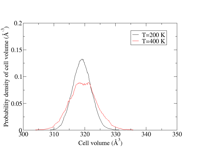
From the figure above, it becomes clear that all local configurations encountered at T = 200 K are already part of the phase space at T = 400 K.
7.2 Input
The input files to run this example are prepared at $TUTORIALS/MD/e07_transferability.
T200/POSCAR
Si16
   1.00000000000000
     5.3624447746476855    5.5400100183731507    0.0700508263882775
    -0.1026916424435065    5.4955175489648100    5.3928259065244042
     5.3656648144783077    0.0000000000074444    5.3656648144915682
   Si
    16
Direct
  0.3212010412955938  1.3122856727003269  0.3107451948534489
  0.3099668704222282  1.3146348632874632  0.8288902495003547
  0.3190369218612182  0.8111634591779978  0.3126913394179140
  0.2964956802844875  0.8343361799802838  0.7984199634929852
 -0.1766690667617155  1.3078055467087799  0.3088469130669039
 -0.2038766002481691  1.3305436458574109  0.8018907176046941
 -0.2003648833919671  0.8282181476495500  0.3026407148396788
 -0.1675550956561834  0.8103292509940945  0.7973543668027023
 -0.0758170429801609  0.9622474667873430 -0.0839264059441386
 -0.0542200245872866  0.9178777992299831  0.4384155478173355
 -0.0619164867449546  0.4239763619295857 -0.0540445435655039
 -0.0538739091128493  0.4506419722481186  0.4087116766428151
 -0.5438457475714482  0.9409158460879290 -0.0753386574943992
 -0.5635400079666790  0.9382672549358126  0.4303926097780276
 -0.5720496423072036  0.4530161102738596 -0.0725936233880037
 -0.5653120928179174  0.4206999169232948  0.4580255784680702
T300/POSCAR.init
Si16
   1.00000000000000
     5.3624447746476855    5.5400100183731507    0.0700508263882775
    -0.1026916424435065    5.4955175489648100    5.3928259065244042
     5.3656648144783077    0.0000000000074444    5.3656648144915682
   Si
    16
Direct
  0.3212010412955938  1.3122856727003269  0.3107451948534489
  0.3099668704222282  1.3146348632874632  0.8288902495003547
  0.3190369218612182  0.8111634591779978  0.3126913394179140
  0.2964956802844875  0.8343361799802838  0.7984199634929852
 -0.1766690667617155  1.3078055467087799  0.3088469130669039
 -0.2038766002481691  1.3305436458574109  0.8018907176046941
 -0.2003648833919671  0.8282181476495500  0.3026407148396788
 -0.1675550956561834  0.8103292509940945  0.7973543668027023
 -0.0758170429801609  0.9622474667873430 -0.0839264059441386
 -0.0542200245872866  0.9178777992299831  0.4384155478173355
 -0.0619164867449546  0.4239763619295857 -0.0540445435655039
 -0.0538739091128493  0.4506419722481186  0.4087116766428151
 -0.5438457475714482  0.9409158460879290 -0.0753386574943992
 -0.5635400079666790  0.9382672549358126  0.4303926097780276
 -0.5720496423072036  0.4530161102738596 -0.0725936233880037
 -0.5653120928179174  0.4206999169232948  0.4580255784680702
T200/INCAR.init
SYSTEM = Si16
ISYM   = 0        ! no symmetry imposed

! MD
IBRION = 0        ! MD (treat ionic degrees of freedom)
NSW    = 10000    ! no of ionic steps
POTIM  = 2.0      ! MD time step in fs

MDALGO = 3                ! Langevin thermostat
LANGEVIN_GAMMA   = 1      ! friction
LANGEVIN_GAMMA_L = 10     ! lattice friction
PMASS  = 10               ! lattice mass
TEBEG  = 200              ! temperature

ISIF   = 3        ! update positions, cell shape and volume

! machine learning
ML_LMLFF  = T
ML_ISTART = 2
T300/INCAR.init
SYSTEM = Si16
ISYM   = 0        ! no symmetry imposed

! MD
IBRION = 0        ! MD (treat ionic degrees of freedom)
NSW    = 10000    ! no of ionic steps
POTIM  = 2.0      ! MD time step in fs

MDALGO = 3                ! Langevin thermostat
LANGEVIN_GAMMA   = 1      ! friction
LANGEVIN_GAMMA_L = 10     ! lattice friction
PMASS  = 10               ! lattice mass
TEBEG  = 300              ! temperature

ISIF   = 3        ! update positions, cell shape and volume

! machine learning
ML_LMLFF  = T
ML_ISTART = 2
LR 1 7
LR 2 7
LR 3 7
LA 2 3 7
LA 1 3 7
LA 1 2 7
LV 7
Gamma-point only
 0
Monkhorst Pack
 1 1 1
 0 0 0
Pseudopotentials of Si.
Click to see the answer!
The lines starting with LR and LV. The lines starting with LA monitor the lattice angles.
7.3 Calculation
Open a terminal, navigate to this example's directory and run VASP by entering the following:
cd $TUTORIALS/MD/e07_*/T200
ln -s $TUTORIALS/MD/e04_MLFF/ML_FFN ML_FF
bash run

cd $TUTORIALS/MD/e07_*/T300
ln -s $TUTORIALS/MD/e04_MLFF/ML_FFN ML_FF
bash run
Extract the lattice vectors and cell volume at each MD step from the subdirectories T*/run* and take the ensemble average.
Click to get a tip!
Write your own python code in the code box below, or use the bash script get_lattice_parameters.sh used in Example 6!
To use bash commands in the code box, you can escape the notebook by starting the line with !. For instance, to show the content of the directory of this example use
! ls e07_transferability
import numpy as np

# extract the lattice vectors and cell volume


# take the average


# print the result
Click to see the answer!
Use the same script as in Example 6 to extract and take the average of the lattice vectors and cell volume over the simulation time!
get_lattice_parameters.sh
#!/bin/bash

if test -f lv.dat
then
  rm lv.dat
  rm lr1.dat lr2.dat lr3.dat lr.dat
fi

step=1

while [ $step -le 3 ]
do
  if test -f run$step/REPORT
  then
    grep LV run$step/REPORT |awk '{print $3}' >> lv.dat
    grep LR run$step/REPORT |awk '{if (NR%3==1) {print $3}}' >> lr1.dat
    grep LR run$step/REPORT |awk '{if (NR%3==2) {print $3}}' >> lr2.dat
    grep LR run$step/REPORT |awk '{if (NR%3==0) {print $3}}' >> lr3.dat
    grep LR run$step/REPORT |awk '{print $3}' >> lr.dat
  fi
  let step=step+1
done

avR1=$(awk 'BEGIN {a=0.} {a+=$1} END {printf("%12.16f\n",a/NR)}' lr1.dat )
avR2=$(awk 'BEGIN {a=0.} {a+=$1} END {printf("%12.16f\n",a/NR)}' lr2.dat )
avR3=$(awk 'BEGIN {a=0.} {a+=$1} END {printf("%12.16f\n",a/NR)}' lr3.dat )
avR=$(awk 'BEGIN {a=0.} {a+=$1} END {printf("%12.16f\n",a/NR)}' lr.dat )

av=$(awk 'BEGIN {a=0.} {a+=$1} END {printf("%12.16f\n",a/NR)}' lv.dat )

echo "            volume:" $av "A^3"
echo "      lat. vect. 1:" $avR1 "A"
echo "      lat. vect. 2:" $avR2 "A"
echo "      lat. vect. 3:" $avR3 "A"
echo "average lat. vect.:" $avR "A"
At T=200K, you will find
            volume: 319.0651260920003551 A^3
      lat. vect. 1: 7.6710057093333308 A
      lat. vect. 2: 7.6712457393333251 A
      lat. vect. 3: 7.6705574270000012 A
average lat. vect.: 7.6709362918889177 A
Finally, at T=300K, the result is
            volume: 319.1915296976661125 A^3
      lat. vect. 1: 7.6726366676666133 A
      lat. vect. 2: 7.6725493826666860 A
      lat. vect. 3: 7.6717844066667205 A
average lat. vect.: 7.6723234856666895 A
Plot the cell volume vs. temperature! Recall that you computed the volume at 400 K in Example 6.
from py4vasp import plot

# fill the list of volume in the same order as the temperature
# volume = [ , , ]
temperature = [200, 300, 400]

plot(temperature, volume, xlabel="T (K)", ylabel="V (ų)")
Click to see the answer!
volume = [319.0651260920003551 , 319.1915296976661125, 319.2866156019985056]
The dependence on the volume ($V$) is approximately linear on this temperature ($T$) range. Make use of this fact to estimate the isotropic expansion coefficient:
$$ \alpha_V = \frac{1}{V} \frac{dV}{dT} $$In other words, determine the derivative from the slope of the cell volume vs. temperature dependence.
alpha_V = 1./volume[2] * (volume[2]-volume[0])/(temperature[2]-temperature[0])
print("Thermal expansion coefficient of Si:", alpha_V)
Click to see the answer!
Thermal expansion coefficient of Si: 3.4685060252297662e-06
However, in the experiment, the linear expansion coefficient is determined considering the length of a lattice vector:
$$ \alpha_L = \frac{1}{L} \frac{dL}{dT}. $$The experimental value for Si is reported to be 2.6e-6 K$^{-1}$ in Y Okada and Y Tokumaru, JAP 56, 314 (1984). Note that for a cubic lattice the following equality holds:
$$ \alpha_L = \alpha_V / 3 $$and use it to determine $\alpha_L$! How does your value compare with experiment?
alpha_L = alpha_V/3
print("Linear expansion coefficient of Si:", alpha_L)
Click to see the answer!
Linear expansion coefficient of Si: 1.1561686750765887e-06 K$^{-1}$
Alternatively, $\alpha_L$ can be computed directly by measuring the lengths of lattice vectors. Here, we can make use of the fact that all three vectors are equivalent and combine them to improve statistics. Plot the average lattice vector vs. temperature, then determine $\alpha_L$ and compare it with the value you obtained through the volume dependence. What are the likely reasons for the difference?
from py4vasp import plot

lattice_vector = [7.6709362918889177, 7.6723234856666895, 7.6730585861110878]
temperature = [200, 300, 400]

alpha_L = 1./lattice_vector[1] * (lattice_vector[2]-lattice_vector[0])/(temperature[2]-temperature[0])
print("Linear expansion coefficient of Si:", alpha_L)

plot(temperature, lattice_vector, xlabel="T (K)", ylabel="a (Å)")
Click to see the answer!
Linear expansion coefficient of Si: 1.3830844242522985e-06 $K^{-1}$
7.4 Questions
- Under what condition is a force field transferable to a new parameter set or system?
- How is the thermal expansion coefficient defined?
- Which file are monitored geometric coordinates written to?