Part 1: An overview of available functionals 
By the end of this tutorial, you will be able to:
- explain what is a hybrid functional
- setup a PBE0 calculation
- compute the band gap
1.1 Task
Compute the band gap of cubic diamond Si using PBE and PBE0.
The computationally most efficient functionals are the local density approximation (LDA), the generalized gradient approximations (GGA) and the meta-GGA functionals. The GGA and meta-GGA functionals are of the semilocal type and a plethora of them have been proposed. The GGA PBE functional, implemented in VASP, is the most commonly used in solid-state physics. However, note that the LDA and GGA functionals do not provide a correct description of the band gap. Whether the Kohn-Sham (KS) orbitals $\psi_{n\mathbf{k}}(\mathbf{r})$ reflect the right physics crucially depends on the type of the used exchange-correlation (xc) functional. In this respect meta-GGA and hybrid functionals are more appropriate for band gap calculation.
Hybrid functionals make up a special category of xc functionals that mix some fraction of Fock exchange into a semilocal functional. This approach is inspired by the well-known Hartree–Fock (HF) method, which is the exact solution for uncorrelated systems. Regarding extended systems, it aims to cure the infamous underestimation of band gaps by the LDA and GGA. The nonlocal Fock potential reads $$\tag{1} V_{\mathrm{x}}^{\mathrm{HF}}\left(\mathbf{r},\mathbf{r}'\right)= -\frac{e^2}{2}\sum_{n\mathbf{k}}f_{n\mathbf{k}} \frac{\psi_{n\mathbf{k}}^{*}(\mathbf{r}')\psi_{n\mathbf{k}}(\mathbf{r})} {\vert \mathbf{r}-\mathbf{r}' \vert}, $$ where $f_{n\mathbf{k}}$ is the occupation of band $n$ and at a specific $\mathbf{k}$ point, $\mathbf{r}$ is the position and $e$ the charge of an electron. Equation (1) depends on the KS orbitals instead of the density and thus, hybrid functionals are not density functionals.
PBE0 is one of the hybrid functionals available in VASP and has the following composition: $$\tag{2} E_{\mathrm{xc}}^{\mathrm{PBE0}} = \frac{1}{4} E_{\mathrm{x}}^{\mathrm{HF}} + \frac{3}{4} E_{\mathrm{x}}^{\mathrm{PBE}} + E_{\mathrm{c}}^{\mathrm{PBE}}. $$ Here, $E_{\mathrm{x}}^{\mathrm{HF}}$ is the Fock exchange energy (the corresponding potential is Equation (1)), while $E_{\mathrm{x}}^{\mathrm{PBE}}$ and $E_{\mathrm{c}}^{\mathrm{PBE}}$ are the PBE exchange and correlation energies, respectively. Compared to many other functionals, PBE0 contains no parameter that were fitted to experimental data.
1.2 Input
The input files to run this example are prepared at $TUTORIALS/hybrids/e01_Si-gap. Check them out!
cubic diamond Si
5.46873
 0.0    0.5     0.5
 0.5    0.0     0.5
 0.5    0.5     0.0
2
Direct
 -0.125 -0.125 -0.125
  0.125  0.125  0.125
SYSTEM = cd Si PBE

GGA    = PE

ISMEAR = -5
LORBIT = 11
PBE0/INCAR
SYSTEM  = cd Si PBE0

GGA     = PE
LHFCALC = T

ISMEAR  = 0
SIGMA   = 0.01

ALGO    = Damped
TIME    = 0.8
K-Points
 0
Gamma
 7 7 7
 0 0 0
Pseudopotential of Si.
The POSCAR file defines the cubic diamond structure of Si.
The INCAR files specify explicitly which xc functional is used. Check the default setting for the GGA tag! Is it necessary to set it in this calculation? PBE0 is activated by LHFCALC, as long as related tags, AEXX, AGGAC and ALDAC, have their default values. How do these tags relate to Equation (2)?
In the PBE calculation, ISMEAR = -5 switches on the tetrahedron method with Blöchl corrections to determine the partial occupations $f_{n\mathbf{k}}$. This smearing yields the smoothest density of states. With LORBIT = 11, VASP writes the projected DOS to the DOSCAR file and the vaspout.h5 file.
In the PBE0 calculation, we use a damped algorithm for the electronic relaxation where the total energy must be variational. This direct optimization algorithm is generally more robust than iterative methods. In many systems, hybrid functionals require this robustness to achieve convergence. Why do we not immediately compute the DOS, like in the PBE calculation?
Click to see the answer!
The Blöchl corrections cause energies not to be variational, thus we use Gaussian smearing with ISMEAR = 0 and SIGMA = 0.01 instead. With the Gaussian smearing, the energies are variational as required for the damped algorithm. After convergence, we perform a single-shot calculation without updating the orbitals (ALGO=None) to get the DOS with the tetrahedron method (ISMEAR = -5) and orbital projections (LORBIT = 11).
The POTCAR file contains the pseudopotential generated for PBE and the KPOINTS file defines an equally-spaced Γ-centered grid of $\mathbf{k}$ points.
The overall settings are such that the precision for the band gap lies within 0.1 eV. What would you need to do in order to confirm this statement and how can you improve the precision?
Click to see the answer!
You would need to perform convergence studies of the cutoff energy and the number of $\mathbf{k}$ points and judge how much the value of the band gap changes.
1.3 Calculation
Open a terminal, navigate to this example's directory and run VASP by entering the following:
cd $TUTORIALS/hybrids/e01_*
vasp_std
Plot the DOS using py4vasp for the PBE calculation.
import py4vasp
pbe_calc = py4vasp.Calculation.from_path("./e01_Si-gap")

pbe_calc.dos.plot()
Where in the DOS plot can you see the band gap?
Click to see the answer!
The electronic band gap is the energy difference between the valence band maximum and the conduction band minimum. In the DOS plot, this corresponds to the energy range without any states in the vicinity of the Fermi energy. Note that the energy axis is aligned to the Fermi energy.
Next, copy the WAVECAR file to the directory of the PBE0 calculation and run VASP there by entering the following:
cd $TUTORIALS/hybrids/e01_*/PBE0
cp ../WAVECAR .
mpirun -np 2 vasp_std
The stdout printed during the calculation shows an additional line with information related to the damped algorithm at each step of the electronic relaxation.
Click to see the answer!
No, generally it does not make sense to compare total energies obtained with different exchange-correlation functionals. Only physical quantities like the band gap can be compared.
import py4vasp
import numpy as np

def gap(calc):
    homo = np.amax(calc.band.to_dict()['bands'][calc.band.to_dict()['occupations'] > 0.5])
    lumo = np.amin(calc.band.to_dict()['bands'][calc.band.to_dict()['occupations'] < 0.5])
    return lumo - homo

pbe_calc = py4vasp.Calculation.from_path("./e01_Si-gap")
pbe0_calc = py4vasp.Calculation.from_path("./e01_Si-gap/PBE0")

for calc in (pbe_calc, pbe0_calc):
    print(f"{str(calc.system):10} {gap(calc):6.3f}")
Which band gap is larger?
Click to see the answer!
The PBE0 band gap (1.84 eV) is larger than the PBE one (0.62 eV). As a general trend in many materials, hybrid functionals lead to larger band gap and partially correct for the underestimation obtained with GGA functionals compared to experiment.
To visualize the PBE0 gap, you can again compute the DOS. Open the INCAR file of your PBE0 calculation and set ISMEAR = -5, ALGO = None, and LORBIT = 11. You may also remove the tag SIGMA and TIME which are not used. Then, restart the calculation with the existing WAVECAR file by entering the following:
cd $TUTORIALS/hybrids/e01_*/PBE0
mpirun -np 2 vasp_std
import py4vasp
pbe_calc = py4vasp.Calculation.from_path("./e01_Si-gap")
pbe0_calc = py4vasp.Calculation.from_path("./e01_Si-gap/PBE0")

pbe_calc.dos.plot().label("PBE") + pbe0_calc.dos.plot().label("PBE0")
Did the overall appearance of the DOS change much compared to the PBE calculation?
Click to see the answer!
The PBE0 DOS is different. Not only is the band gap enlarged, but also the relative energy between bands and the bands width are different. These subtle changes can crucially influence the properties of the material.
By the end of this tutorial, you will be able to:
- use the B3LYP functional
- use the HF method
- explain the limitations of HF and B3LYP
2.1 Task
Compute the band gap of Ar using PBE, B3LYP and HF.
B3LYP was originally designed to describe molecular properties and is a semiempirical hybrid functional. Semiempirical implies that parameters were fitted to reproduce experimental results for properties like the atomization energies, electron-proton affinities and ionization potentials for atoms and molecules of a test set. The empirical parameters are the ones that multiply the various components of the B3LYP functional:
$$\tag{1 a} E_{\mathrm{xc}}^{\mathrm{B3LYP}} = E_{\mathrm{x}}^{\mathrm{B3LYP}} + E_{\mathrm{c}}^{\mathrm{B3LYP}} $$$$ \tag{1 b} E_{\mathrm{x}}^{\mathrm{B3LYP}} = 0.8 E_{\mathrm{x}}^{\mathrm{LDA}} + 0.2 E_{\mathrm{x}}^{\mathrm{HF}} + 0.72 \Delta E_{\mathrm{x}}^{\mathrm{B88}}. $$$$ \tag{1 c} E_{\mathrm{c}}^{\mathrm{B3LYP}} = 0.19 E_{\mathrm{c}}^{\mathrm{VWN3}} + 0.81 E_{\mathrm{c}}^{\mathrm{LYP}}. $$In a HF calculation, the exchange consists of the full Fock exchange (AEXX = 1) and no correlation effects are considered ($E_{\mathrm{c}}=0$).
B3LYP and other unscreened functionals inherit a fundamental flaw of the HF method—its failure in the limit of the homogeneous electron gas. This failure originates from a singularity of the Fourier transform of the Fock potential at $\mathbf{q}=0$
$$\tag{2} V_{\mathrm{x}}^{\mathrm{HF}}\left(\mathbf{q}\right)= -\frac{4\pi e^2}{2}\sum_{n\mathbf{k}}f_{n\mathbf{k}} \frac{\psi_{n\mathbf{k}}^{*}(\mathbf{r}')\psi_{n\mathbf{k}}(\mathbf{r})} { \mathbf{q} }~. $$This causes a complete suppression of itinerant states. In other words, the HF method and hybrid functionals are not recommended for systems with significant itinerant character, such as metals and small gap semiconductors, see Paier et al. (2007).
Here, let us investigate the band gap of Ar, which is found to have a large band gap of 14.4 eV in experiment!
2.2 Input
The input files to run this example are prepared at $TUTORIALS/hybrids/e02_Ar-gap. Check them out!
Ar Fm-3m
1.0
  3.454253 0.000000 1.994314
  1.151418 3.256701 1.994314
  0.000000 0.000000 3.988628
  Ar
  1
direct
  0.000000 0.000000 0.000000 Ar
SYSTEM = Ar

ISMEAR = -5
ENCUT  = 300

LORBIT = 11
HF/INCAR
SYSTEM  = Ar HF

LHFCALC = T
AEXX    = 1

ISMEAR  = 0
SIGMA   = 0.01
ENCUT   = 300

ALGO    = Damped
TIME    = 0.4
B3LYP/INCAR
SYSTEM = Ar B3LYP

GGA     = B3
LHFCALC = T
AEXX    = 0.2
AGGAX   = 0.72
AGGAC   = 0.81
ALDAC   = 0.19

ISMEAR  = 0
SIGMA   = 0.01

ALGO    = Damped
TIME    = 0.4
K-Points
 0
Gamma
4  4  4
0  0  0
Pseudopotential of Ar.
The POSCAR file defines the face-centered-cubic Ar crystal.
The first INCAR file runs a PBE calculation. Check the meaning of unfamiliar tags on the VASP Wiki!
In the HF INCAR file, the evaluation of Fock exchange is switched on using the LHFCALC tag and the fraction of HF is set by AEXX. So only Fock exchange and no semilocal functional exchange-correlation is used. Recall the meaning of the remaining tags! What are the default values of GGA, AGGAX, AGGAC and ALDAC here?
2.3 Calculation
Open a terminal, navigate to this example's directory and run VASP by entering the following:
cd $TUTORIALS/hybrids/e02_*
vasp_std
You can visualize the DOS of the PBE calculation with py4vasp!
import py4vasp
pbe_calc = py4vasp.Calculation.from_path("./e02_Ar-gap")

pbe_calc.dos.plot()
import py4vasp
import numpy as np

def gap(calc):
    homo = np.amax(calc.band.to_dict()['bands'][calc.band.to_dict()['occupations'] > 0.5])
    lumo = np.amin(calc.band.to_dict()['bands'][calc.band.to_dict()['occupations'] < 0.5])
    return lumo - homo

pbe_calc = py4vasp.Calculation.from_path( "./e02_Ar-gap")
hf_calc = py4vasp.Calculation.from_path( "./e02_Ar-gap/HF")
b3lyp_calc = py4vasp.Calculation.from_path( "./e02_Ar-gap/B3LYP")

for calc in [pbe_calc, hf_calc, b3lyp_calc]:
    print(f"{str(calc.system):10} {gap(calc):6.3f}")
2.4 Questions
- Which class of systems do the PBE0 and B3LYP functionals and HF method fail to describe well? Why?
- What does the AGGAC tag control?
By the end of this tutorial, you will be able to:
- understand the fundamentals of screened hybrid functionals
- explain the basic assumptions taken by the HSE06 functional
- optimize the fraction of exchange and the screening length for the band gap
3.1 Task
Optimize the fraction of Fock exchange in a screened hybrid functional in order to reproduce the experimental band gap of MgO.
Screened hybrid functionals decompose the $1/r$ dependence of the Fock exchange into a short-range (SR) and a long-range (LR) contribution introducing a screening parameter $\mu$:
$$\tag{1} E_{\mathrm{xc}}^{\mathrm{screened}} = \frac{1}{4} E_{\mathrm{x}}^{\mathrm{HF,SR}}(\mu) + \frac{3}{4} E_{\mathrm{x}}^{\mathrm{PBE,SR}}(\mu) + E_{\mathrm{x}}^{\mathrm{PBE,LR}}(\mu) + E_{\mathrm{c}}^{\mathrm{PBE}}. $$The SR limit is identical to the PBE0 functional. But by truncating the LR contribution, screened hybrid functionals avoid the singularity in the Fock exchange. This singularity is responsible for the suppression of all metallic states. Additionally, screened hybrid functionals allow to reduce the computational cost by downsampling.
In solid-state physics, one commonly used functional is HSE06. In this functional, the screening parameter was empirically optimized for a value of μ = 0.2 Å$^{−1}$. The corresponding interaction range $2 / \mu \approx 10$ Å typically reaches a few nearest neighbors. In VASP, you control the screening length by the HFSCREEN tag.
The gap size still crucially depends on the fraction of Fock exchange introduced. Let us take a practical approach here and optimize the mixing to reproduce the experimental band gap of MgO of 7.7 eV! Note that you sacrifice the predictive power of a first-principles approach here. Instead, this approach is closer to model physics where you want to get qualitative insights into the system. Please do not refer to this fitted functional as HSE as it is occasionally done in the literature. HSE06 corresponds only to AEXX = 0.25 and HFSCREEN = 0.2.
3.2 Input
The input files to run this example are prepared at $TUTORIALS/hybrids/e03_MgO-gap-optimization. Check them out!
MgO Fm-3m (No. 225)
1.0
  2.606553 0.000000 1.504894
  0.868851 2.457482 1.504894
  0.000000 0.000000 3.009789
  Mg O
  1 1
direct
  0.000000 0.000000 0.000000 Mg
  0.500000 0.500000 0.500000 O
SYSTEM = MgO

ENCUT  = 500
ISMEAR = -5

LORBIT = 11
screened_hybrid/INCAR
SYSTEM   = MgO HSE06

ENCUT    = 500
ISMEAR   = 0
SIGMA    = 0.01

LHFCALC  = T
HFSCREEN = 0.2
AEXX     = 0.25

ALGO     = Damped
TIME     = 0.4
K-Points
 0
Gamma centered
 4  4  4
 0  0  0
Pseudopotential of Mg, and O.
3.3 Calculation
Open a terminal, navigate to this example's directory and run VASP by entering the following:
cd $TUTORIALS/hybrids/e03_*
vasp_std
The band gap with PBE can be seen in the DOS. Plot it using py4vasp!
import py4vasp
pbe_calc = py4vasp.Calculation.from_path("./e03_MgO-gap-optimization")

pbe_calc.dos.plot()
Then, in the screened_hybrid directory run a loop over different values of the fraction of HF exchange AEXX by entering the following:
cd $TUTORIALS/hybrids/e03_*/screened_hybrid
bash loop_aexx.sh
loop_aexx.sh
for aexx in 0.40 0.45 0.50 0.55
do
vasp_rm
cp ../WAVECAR .
cat > INCAR << EOF
SYSTEM   = MgO $aexx

ENCUT    = 500
ISMEAR   = 0
SIGMA    = 0.01

LHFCALC  = T
HFSCREEN = 0.2
AEXX     = $aexx

ALGO     = Damped
TIME     = 0.4
EOF

mpirun -np 2 vasp_std

mkdir aexx$aexx
cp vaspout.h5 aexx$aexx/.
done
import py4vasp
import numpy as np

def gap(calc):
    homo = np.amax(calc.band.to_dict()['bands'][calc.band.to_dict()['occupations'] > 0.5])
    lumo = np.amin(calc.band.to_dict()['bands'][calc.band.to_dict()['occupations'] < 0.5])
    return lumo - homo

for aexx in ['0.40', '0.45', '0.50', '0.55']:
    calc = py4vasp.Calculation.from_path(f"./e03_MgO-gap-optimization/screened_hybrid/aexx{aexx}")
    print(f"AEXX:  {aexx},  Band gap (eV): {gap(calc):6.3f}")
Click to see the answer!
The optimal AEXX should be between 0.45 and 0.50.
Next, we use a value of AEXX close to the optimum and vary the screening HFSCREEN!
bash loop_hfscreen.sh
loop_hfscreen.sh
for hfscreen in 0.15 0.20 0.25 0.30
do
vasp_rm
cp ../WAVECAR .
cat > INCAR << EOF
SYSTEM   = MgO $hfscreen

ENCUT    = 500
ISMEAR   = 0
SIGMA    = 0.01

LHFCALC  = T
HFSCREEN = $hfscreen
AEXX     = 0.5

ALGO     = Damped
TIME     = 0.4
EOF

mpirun -np 2 vasp_std

mkdir hfscreen$hfscreen
cp vaspout.h5 hfscreen$hfscreen/.
done
Is the result sensitive to the fraction of screening?
import py4vasp
import numpy as np

def gap(calc):
    homo = np.amax(calc.band.to_dict()['bands'][calc.band.to_dict()['occupations'] > 0.5])
    lumo = np.amin(calc.band.to_dict()['bands'][calc.band.to_dict()['occupations'] < 0.5])
    return lumo - homo

for hfscreen in ['0.15', '0.20', '0.25', '0.30']:
    calc = py4vasp.Calculation.from_path(f"./e03_MgO-gap-optimization/screened_hybrid/hfscreen{hfscreen}")
    print(f"HFSCREEN: {hfscreen}, Band gap (eV): {gap(calc):6.3f}")
Click to see the answer!
Yes, a shorter screening length increases the amount of Fock exchange and consequently the band gap.
3.4 Questions
- What does the HFSCREEN tag control?
- Is PBE0 range dependent?
- What contributions are part of the HSE06 functional?
By the end of this tutorial, you will be able to:
- compute the band structure using a hybrid functional
4.1 Task
Perform an HSE06 calculation for CaS, compute the band structure and the band gap.
The band structure is computed along so-called high-symmetry lines that connect high-symmetry points in the first Brillouin zone. These are of special interest, e.g., due to symmetry imposed degeneracy. In many cases, extrema form along these lines so that the $\mathbf{k}$ points which constitute the valence band maximum and conduction band minimum (also called HOMO and LUMO) can be identified. If they are at the same $\mathbf{k}$ point, the band gap is called direct, otherwise it is indirect.
There are a couple of tools that help you pick a $\mathbf{k}$ path. One of them is SeeK-path, which accepts POSCAR files as an input and is accessible via a web interface. You can download this example's POSCAR and try generating your own KPOINTS file!
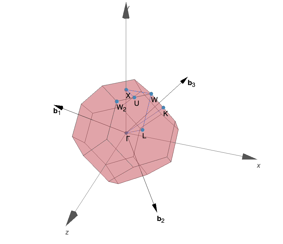
Figure 1: First Brillouin zone of CaS generated by SeeK-path.
4.2 Input
The input files to run this example are prepared at $TUTORIALS/hybrids/e04_CaS-band. Check them out!
CaS Fm-3m (No.225)
1.0
  3.500468 0.000000 2.020996
  1.166823 3.300273 2.020996
  0.000000 0.000000 4.041992
Ca S
 1 1
direct
  0.000000 0.000000 0.000000 Ca
  0.500000 0.500000 0.500000 S
SYSTEM = CaS

ENCUT  = 500
ISMEAR = -5

LORBIT = 11
band/INCAR
SYSTEM = CaS band

ENCUT  = 500
ISMEAR = 0
ISIGMA = 0.01

ICHARG = 11
LORBIT = 11
HSE06/INCAR
SYSTEM   = CaS HSE06

ENCUT    = 500
ISMEAR   = 0
SIGMA    = 0.01

LHFCALC  = T
HFSCREEN = 0.2

ALGO     = Damped
TIME     = 0.4
HSE06/band/INCAR
SYSTEM   = CaS HSE06 band

ENCUT    = 500
ISMEAR   = 0
SIGMA    = 0.01
NELMIN   = 4

LHFCALC  = T
HFSCREEN = 0.2
LORBIT   = 11
K-Points
 0
Gamma
 6 6 6
 0 0 0
band/KPOINTS
Special k-points for band structure
10  ! intersections
line-mode
reciprocal
    0.5000000000     0.5000000000     0.5000000000     L
    0.5000000000     0.2500000000     0.7500000000     W

    0.5000000000     0.2500000000     0.7500000000     W
    0.5000000000     0.0000000000     0.5000000000     X

    0.5000000000     0.0000000000     0.5000000000     X
    0.0000000000     0.0000000000     0.0000000000     GAMMA

    0.0000000000     0.0000000000     0.0000000000     GAMMA
    0.5000000000     0.5000000000     0.5000000000     L
HSE06/KPOINTS
K-Points
 0
Gamma
 6 6 6
 0 0 0
HSE06/band/KPOINTS
Click to see the file!
Explicit k-points list for band structure
53 ! Total number of k-points = 37 (band structure) + 16 (IBZKPT file)
reciprocal
    0.00000000000000    0.00000000000000    0.00000000000000             1
    0.16666666666667   -0.00000000000000    0.00000000000000             8
    0.33333333333333   -0.00000000000000    0.00000000000000             8
    0.50000000000000   -0.00000000000000    0.00000000000000             4
    0.16666666666667    0.16666666666667    0.00000000000000             6
    0.33333333333333    0.16666666666667    0.00000000000000            24
    0.50000000000000    0.16666666666667    0.00000000000000            24
   -0.33333333333333    0.16666666666667    0.00000000000000            24
   -0.16666666666667    0.16666666666667    0.00000000000000            12
    0.33333333333333    0.33333333333333    0.00000000000000             6
    0.50000000000000    0.33333333333333    0.00000000000000            24
   -0.33333333333333    0.33333333333333    0.00000000000000            12
    0.50000000000000    0.50000000000000    0.00000000000000             3
    0.50000000000000    0.33333333333333    0.16666666666667            24
   -0.33333333333333    0.33333333333333    0.16666666666667            24
   -0.33333333333333    0.50000000000000    0.16666666666667            12
  0.500000  0.500000  0.500000      0  L
  0.500000  0.472222  0.527778      0
  0.500000  0.444444  0.555556      0
  0.500000  0.416667  0.583333      0
  0.500000  0.388889  0.611111      0
  0.500000  0.361111  0.638889      0
  0.500000  0.333333  0.666667      0
  0.500000  0.305556  0.694444      0
  0.500000  0.277778  0.722222      0
  0.500000  0.250000  0.750000      0  W
  0.500000  0.222222  0.722222      0
  0.500000  0.194444  0.694444      0
  0.500000  0.166667  0.666667      0
  0.500000  0.138889  0.638889      0
  0.500000  0.111111  0.611111      0
  0.500000  0.083333  0.583333      0
  0.500000  0.055556  0.555556      0
  0.500000  0.027778  0.527778      0
  0.500000  0.000000  0.500000      0  X
  0.444444  0.000000  0.444444      0
  0.388889  0.000000  0.388889      0
  0.333333  0.000000  0.333333      0
  0.277778  0.000000  0.277778      0
  0.222222  0.000000  0.222222      0
  0.166667  0.000000  0.166667      0
  0.111111  0.000000  0.111111      0
  0.055556  0.000000  0.055556      0
  0.000000  0.000000  0.000000      0  Gamma
  0.055556  0.055556  0.055556      0
  0.111111  0.111111  0.111111      0
  0.166667  0.166667  0.166667      0
  0.222222  0.222222  0.222222      0
  0.277778  0.277778  0.277778      0
  0.333333  0.333333  0.333333      0
  0.388889  0.388889  0.388889      0
  0.444444  0.444444  0.444444      0
  0.500000  0.500000  0.500000      0  L
Pseudopotential of Ca, and S.
The POSCAR file contains the face centered cubic structure of CaS.
The INCAR files should contain only familiar tags. Otherwise, please look up their meaning on the VASP Wiki!
The self-consistent calculations of both, PBE and HSE06, are performed on a uniform $\mathbf{k}$ mesh, that is defined in the KPOINTS file. Then, the band/KPOINTS file for the PBE band-structure is written using the line mode. This is an easy way to generate $\mathbf{k}$ points along a path.
For the band-structure calculation using a hybrid functional, you need both, the $\mathbf{k}$ points along a high-symmetry path and a uniform $\mathbf{k}$ mesh to evaluate the Fock exchange energy. This is why the HSE06/band/KPOINTS file comprises 16 irreducible $\mathbf{k}$ points with their corresponding weights to span the first Brillouin zone, and 37 $\mathbf{k}$ points with zero weight to define the same path as used for the PBE bands.
4.3 Calculation
Open a terminal, navigate to this example's directory and run VASP by entering the following:
cd $TUTORIALS/hybrids/e04_*
vasp_std
Next, compute the band structure of the PBE calculation by entering the following:
cd $TUTORIALS/hybrids/e04_*/band
cp ../CHGCAR .
vasp_std
You can plot the band structure using py4vasp. Use the documentation to learn how to plot the character of a band! Then, replace the character ? of my_calc_band.plot by what is appropriate.
import py4vasp
my_calc = py4vasp.Calculation.from_path("./e04_CaS-band/band")

my_calc.band.plot?
Navigate to the HSE06 directory and run VASP by entering the following:
cd $TUTORIALS/hybrids/e04_*/HSE06
cp ../WAVECAR .
mpirun -np 2 vasp_std
While this is running, compare the HSE06/band/KPOINTS file with the IBZKPT file and the reciprocal coordinates in the band/OUTCAR file of the PBE calculation! What $\mathbf{k}$ points are specified? How are the weights determined.
Click to see the answer!
The $\mathbf{k}$ points associated with the band structure are the same in both cases. For the hybrid functional, we additionally need to specify a uniform $\mathbf{k}$ mesh on which the Fock energy is evaluated also for during the band-structure calculation. That is why the weight associated with the uniform $\mathbf{k}$ mesh are chosen in accordance with the irreducible Brillouin zone and the weight of the band-structure $\mathbf{k}$ points is zero.
Click to see the answer!
Since we restart the calculation from an existing WAVECAR file, the total energy of the system is already converged. Therefore VASP will stop updating the orbitals after NELMIN iterations. To obtain the eigenvalues, the Kohn-Sham Hamiltonian is diagonalized in the basis of these orbitals. The orbitals at the additional $\mathbf{k}$ points may not be sufficiently converged yet, so that the basis is not good enough to get accurate eigenvalues. If that happens you will see jumps in the band structure. To avoid this, we ensure that at least four updates are done.
Let us look at the band structure with the hybrid functional now. You will see all the $\mathbf{k}$ points, also the one from the regular grid. Please use the interactive features to zoom to the area between the two L-point labels.
import py4vasp
my_calc = py4vasp.Calculation.from_path("./e04_CaS-band/HSE06/band")

my_calc.band.plot()
If you look closely at the conduction band, slight kinks can still be seen. This can be improved by running a longer run (NELMIN) or using more bands (NBANDS).
Finally, compute the band gap and compare the value to the band structure. Is the band gap direct or indirect? At which $\mathbf{k}$ point? How does it compare to the experimental value of 5.4 eV?
import py4vasp
import numpy as np

def gap(calc):
    homo = np.amax(calc.band.to_dict()['bands'][calc.band.to_dict()['occupations'] > 0.5])
    lumo = np.amin(calc.band.to_dict()['bands'][calc.band.to_dict()['occupations'] < 0.5])
    return lumo - homo

pbe_calc = py4vasp.Calculation.from_path("./e04_CaS-band/band")
hse06_calc = py4vasp.Calculation.from_path("./e04_CaS-band/HSE06/band")

for calc in (pbe_calc, hse06_calc):
    print(f"{str(calc.system):15} {gap(calc):6.3f}")
Click to see the answer!
The band gap is indirect, since the LUMO is at the X point and the HOMO is at the Γ point.
4.4 Questions
- What steps are necessary to compute the band structure of systems using hybrid functionals?
- Why do the $\mathbf{k}$ points associated with the high-symmetry points have zero weight in this example?
- What is an indirect band gap?