Part 1: Silicon as a typical bulk material 
By the end of this tutorial, you will be able to:
- recognize a face-centered-cubic (fcc) structure by looking at the lattice matrix
- create a Γ-centered $\mathbf{k}$ mesh
- find the lattice constant of an fcc structure by manually performing density-functional-theory (DFT) calculations at different volumes of the unit cell
- use the universal scaling factor in the POSCAR file
1.1 Task
Perform multiple DFT calculations for fcc silicon at different lattice constants and find the total energy minimum w.r.t. the lattice constant.
There are 14 Bravais lattices, that are obtained by combining one of the seven lattice systems (triclinic, monoclinic, orthorhombic, tetragonal, hexagonal and cubic) with one of the centering types (primitive, base-centered, body-centered and face-centered). A primitive cell is the smallest building block of a periodic system, i.e., of a bulk crystal. It is spanned by three lattice vectors $\mathbf{a}$, $\mathbf{b}$ and $\mathbf{c}$, with certain properties, for instance, the enclosed angle, depending on the lattice system.
Additionally, if you take the Fourier transform of the real-space lattice, your system is transformed into $\mathbf{k}$ space, also called reciprocal space. The first Brillouin zone is a uniquely defined primitive cell in reciprocal space. A computationally important concept is the irreducible Brillouin zone, which is the first Brillouin zone reduced by all symmetry operations in the crystallographic point group. Another concept worth mentioning is the use of high-symmetry lines and points, which are of special interest due to symmetry-imposed degeneracies in the electronic band structure. These points have special names, such as the Γ-point at the origin of the Brillouin zone.
1.2 Input
fcc Si
a
 0.5 0.5 0.0
 0.0 0.5 0.5
 0.5 0.0 0.5
   1
cartesian
0 0 0
System = fcc Si

ISTART = 0    ! start from scratch
ICHARG = 2    ! superposition of atomic charge densities

ENCUT  = 240  ! energy cutoff
ISMEAR = 0    ! Gaussian smearing
SIGMA = 0.1   ! broadening
K-Points
 0
Monkhorst Pack
 11 11 11
 0  0  0
Pseudopotential of Si.
Regarding the POSCAR file:
The conventional cell of an fcc structure shows all symmetries, that correspond to a cube ($a=b=c$) with additional sites in the center of each face. But there is a choice of lattice vectors, which represents the same structure in a smaller unit cell. That is the primitive unit cell. A symmetric choice of primitive lattice vectors is
$$\tag{1a}
\mathbf{a} = \frac{a}{2} \left( \hat{\mathbf{x}} + \hat{\mathbf{y}} \right)
$$
$$\tag{1b}
\mathbf{b} = \frac{a}{2} \left( \hat{\mathbf{y}} + \hat{\mathbf{z}} \right)
$$
$$\tag{1c}
\mathbf{c} = \frac{a}{2} \left( \hat{\mathbf{z}} + \hat{\mathbf{x}} \right).
$$
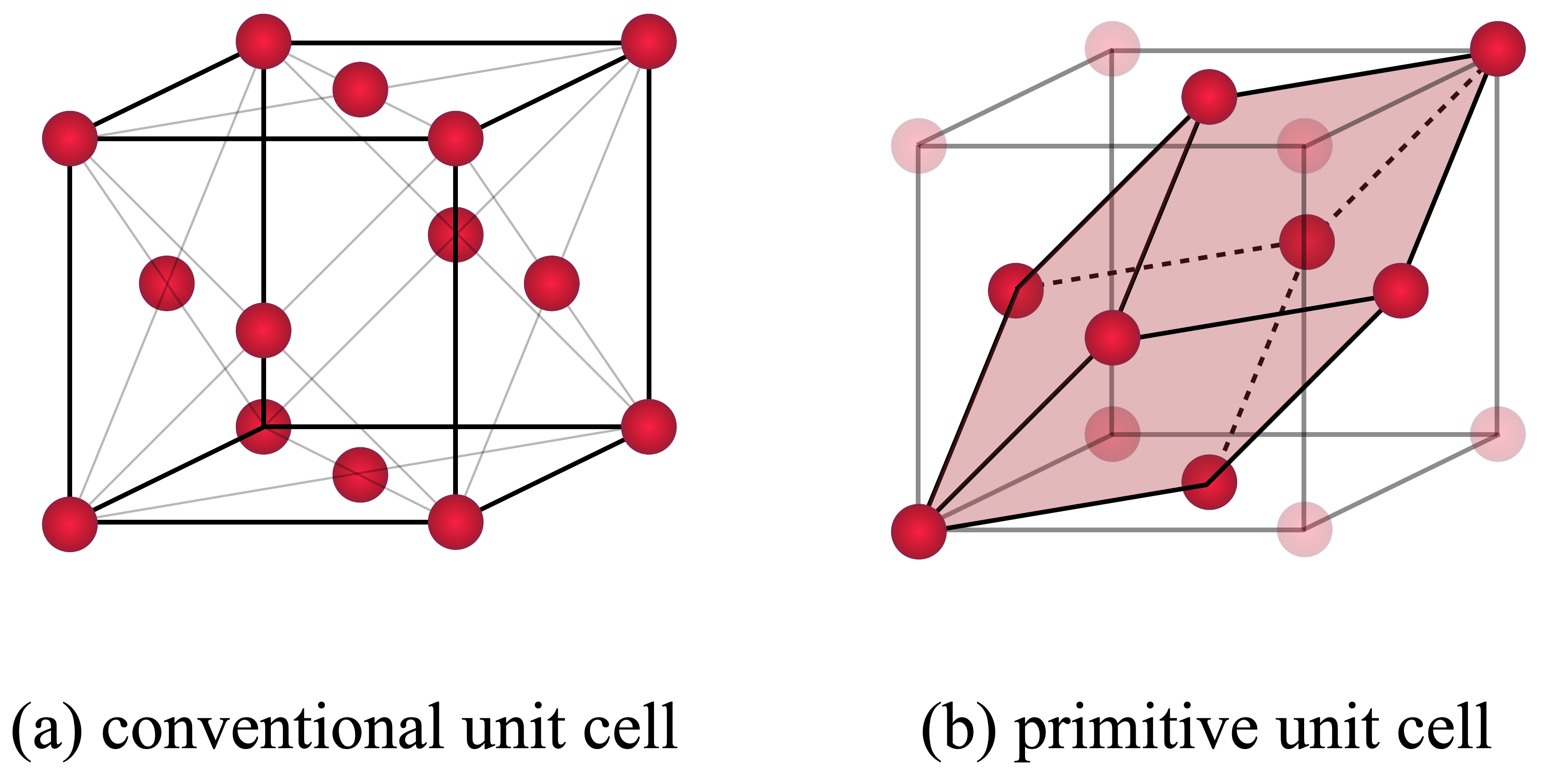
Ask yourself, how many atoms comprise the conventional unit cell and how many atoms comprise the primitive unit cell?
Click to see the answer!
In the conventional unit cell there are 8 vertices and 6 faces, where atoms are shared by multiple cells so that they contribute with $1/8$ and $1/2$ respectively. In total this yields $$ n = 8 \cdot \frac{1}{8} + 6 \cdot \frac{1}{2} = 4 $$ atoms in the conventional unit cell. Similarly, you will find 1 atom in the primitive unit cell.
Click to see the answer!
Line 3, 4, 5 correspond to $\mathbf{b}/a$, $\mathbf{c}/a$ and $\mathbf{a}/a$, respectively. Then, Equations $(1a)$-$(1c)$ are recovered by interpreting the universal scaling parameter in line 2 as lattice constant.
Regarding the INCAR file, the default setting for VASP is to look for an existing WAVECAR file in the current directory and restart the calculation from there. Thus, it is possible to delete the WAVECAR file to start a fresh calculation. It is also possible to control the behavior explicitly by means of the ISTART tag and ICHARG tag. Check out the meaning of those tags on the VASP Wiki!
How is the charge density initialized? What is the energy cutoff? What would the energy cutoff be, if it were not set in the INCAR file?
Click to see the answer!
- Initial charge density from overlapping atoms.
- Energy cutoff of 240 eV from POTCAR file.
Regarding the KPOINTS file, the Monkhorst Pack mode is used to generate a $\mathbf{k}$ mesh with equally spaced $\mathbf{k}$ points. The odd number of $\mathbf{k}$ points in each direction results in a Γ-centered $\mathbf{k}$ mesh.
1.3 Calculation
Open a terminal and navigate to this example's directory by entering the following:
cd $TUTORIALS/bulk/e01_*
In order to run VASP at different lattice constants, the POSCAR file needs to be adjusted. For each run replace a with 3.5 to 4.3 with step size 0.1 and run VASP with
mpirun -np 2 vasp_std
After VASP ran, the OSZICAR file contains a summary stating the total free energy. Run multiple VASP calculations at different lattice constants and store the result in loop_lattice_constant.dat!
Click to see the provided script to do the job!
rm -f loop_lattice_constant.dat
for a in  3.5 3.6 3.7 3.8 3.9 4.0 4.1 4.2 4.3
do
cat > POSCAR << EOF
fcc:
$a
 0.5 0.5 0.0
 0.0 0.5 0.5
 0.5 0.0 0.5
1
cartesian
0 0 0
EOF

mpirun -np 2 vasp_std

en=$(awk '/F=/ {print $0}' OSZICAR)
echo $a $en  >> loop_lattice_constant.dat
done
In this example's directory enter the following into the terminal to run the above script:
bash loop_lattice_constant.sh
Plot the data collected in loop_lattice_constant.dat!
Click to see the answer!
You can use the gnuplot script loop_lattice_constant.gp, that is prepared in this example's directory:
set term png
set output "loop_lattice_constant.png"

set title "lattice constant of fcc Si"
set xlabel "lattice constant [Angstrom]"
set ylabel "total free energy"

plot "loop_lattice_constant.dat" using 1:4 w lp
It can be executed by entering the following into the terminal in this example's directory:
gnuplot loop_lattice_constant.gp
Then, open loop_lattice_constant.png from the file browser. You may need to refresh the file browser.
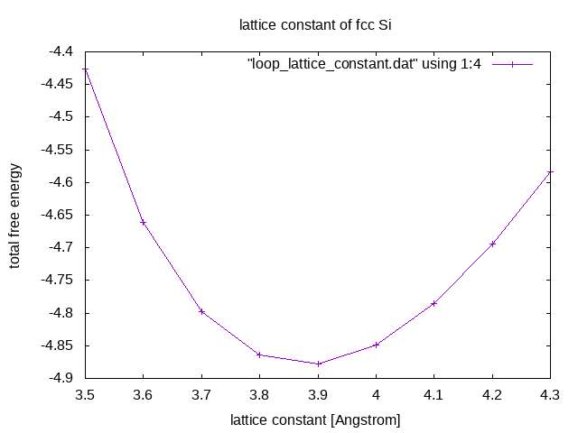
Among the tested parameters, at what lattice constant is the total energy minimized? Write the POSCAR file with the optimal lattice constant and copy it to the next example's directory!
Click to see the answer!
Among the tested parameters, the total energy is minimized at 3.9 Å. Thus, the final calculation is run with:
fcc Si
3.9            ! scaling parameter
 0.5 0.5 0.0
 0.0 0.5 0.5
 0.5 0.0 0.5
   1
cartesian
0 0 0
cp POSCAR ../e02_*/.
1.4 Questions
- What is the definition of the Γ point?
- Write down another form of an fcc lattice matrix of a primitive unit cell!
- Does the conventional fcc unit cell comprise nonprimitive translations?
By the end of this tutorial, you will be able to:
- extract the number of irreducible $\mathbf{k}$ points from the VASP output
- approximate how much computational effort is saved by employing the point-group symmetry of the reciprocal lattice
- state the task that the Monkhorst–Pack method addresses
- set ISMEAR appropriate to compute the density of states (DOS)
- plot the DOS using py4vasp
- set the NEDOS, EMIN and EMAX tags
2.1 Task
Perform a DFT calculation with the appropriate number of $\mathbf{k}$ points and energy broadening in order to plot the DOS of fcc Si.
Locally, the system may obey one of 32 crystallographic point groups, which are discrete rotational symmetries of crystals. In order to reduce the computational effort, VASP searches and takes advantage of these symmetries of the system by default. What's more, in reciprocal space, the system obeys a certain translative symmetry group specified by the Bravais lattices. This nonlocal symmetry is implicitly defined by imposing periodic boundary conditions onto the structure specified in the POSCAR file and it results in a point-group symmetry of the reciprocal lattice. Again, VASP searches and takes advantage of these symmetries, but it is crucial that the $\mathbf{k}$ mesh specified in KPOINTS also conserves the same point-group symmetry of the reciprocal lattice as defined by the structure specified in the POSCAR file.
For more information read the following articles: Symmetry reduction of the mesh, KPOINTS.
2.2 Input
The input files to run this example are prepared at $TUTORIALS/bulk/e02_fcc-Si-DOS. Check them out!
Click to see the answer!
ISMEAR = -5 calls the tetrahedron method with Blöchl corrections. Mind that this method is not variational with respect to partial occupancies and yields erroneous forces and stress for systems with partially filled bands. Therefore, it should not be used when performing geometry optimization in metals! LORBIT = 11 allows the DOSCAR file to be written.
Concerning the KPOINTS file, one scheme to automatically generate a $\mathbf{k}$ mesh in VASP is the Monkhorst–Pack method. In a nutshell, based on the point group symmetry of the reciprocal lattice, some $\mathbf{k}$ points of the first Brillouin zone are found to be equivalent. With this, it is possible to define a set of irreducible $\mathbf{k}$ points and weights. The weight of an irreducible $\mathbf{k}$ point indicates how many equivalent $\mathbf{k}$ points exist in the first Brillouin zone. This allows replacing any sum over all $\mathbf{k}$ points of the first Brillouin zone by a sum over all irreducible $\mathbf{k}$ points with these weights.
Γ-centered $N\times N \times N$ Monkhorst-Pack grids guarantee that the reciprocal lattice and the generating lattice obey the same Bravais lattices. But depending on your calculation you may not need the same number of $\mathbf{k}$ points in each direction. And by varying the number of $\mathbf{k}$ points in each direction, you can still end up with a $\mathbf{k}$ mesh that is inconsistent with your Bravais lattices. For more information read the following articles: Monkhorst Pack, Symmetry reduction of the mesh, KPOINTS.
Are the $\mathbf{k}$ points equally spaced? Is the $\mathbf{k}$ mesh Γ-centered? Why (not)? Compare the specified $\mathbf{k}$ mesh with the one used in the previous example. What changed?
Click to see the answer!
The Monkhorst Pack mode is used to generate a $\mathbf{k}$ mesh with equally spaced $\mathbf{k}$ points. The odd number of $\mathbf{k}$ points in each direction results in a Γ-centered $\mathbf{k}$ mesh. We significantly increase the $\mathbf{k}$-mesh density to yield a smooth DOS. For the geometry relaxation in Example 1 fewer $\mathbf{k}$ points are sufficient to compute the total energy.
2.3 Calculation
Open a terminal, navigate to this example's directory and run VASP by entering the following:
cd $TUTORIALS/bulk/e02_*
mpirun -np 2 vasp_std
Check the OUTCAR file to find at how many $\mathbf{k}$ points the Kohn–Sham orbitals and eigenenergies are computed!
Click to see the answer!
The following is an excerpt of OUTCAR file, in which the $\mathbf{k}$ mesh is discussed.
KPOINTS: K-Points
Automatic generation of k-mesh.
Grid dimensions read from file:
generate k-points for: 15 15 15
Generating k-lattice:
Cartesian coordinates Fractional coordinates (reciprocal lattice)
0.017094017 0.017094017 -0.017094017 0.066666667 -0.000000000 -0.000000000
-0.017094017 0.017094017 0.017094017 -0.000000000 0.066666667 0.000000000
0.017094017 -0.017094017 0.017094017 0.000000000 0.000000000 0.066666667
Length of vectors
0.029607706 0.029607706 0.029607706
Shift w.r.t. Gamma in fractional coordinates (k-lattice)
0.000000000 0.000000000 0.000000000
TETIRR: Found 484 inequivalent tetrahedra from 20250
Subroutine IBZKPT returns following result:
===========================================
Found 120 irreducible k-points:
Following reciprocal coordinates:
Coordinates Weight
0.000000 0.000000 0.000000 1.000000
0.066667 -0.000000 -0.000000 8.000000
0.133333 0.000000 0.000000 8.000000
0.200000 0.000000 0.000000 8.000000
0.266667 0.000000 -0.000000 8.000000
0.333333 -0.000000 -0.000000 8.000000
...
It states that 120 irreducible $\mathbf{k}$ points were found and they are listed below with their respective weight. The weight indicates how many equivalent $\mathbf{k}$ points exist in the full first Brillouin zone. Any sum over all 3375 $\mathbf{k}$ points of the first Brillouin zone, is replaced by a sum over all 120 irreducible $\mathbf{k}$ points with these weights.
Plot the DOS of fcc Si with py4vasp:
import py4vasp
mycalc = py4vasp.Calculation.from_path( "./e02_fcc-Si-DOS" )
mycalc.dos.plot()
Here, the DOS is shifted such that in the plot the Fermi energy is at 0 eV. Let us now plot the DOS in the vicinity of the Fermi energy with a higher resolution! That means we need to recompute the DOS with more points in that energy range, for instance -15 eV to 2 eV. Open your current OUTCAR file and find the Fermi energy of the converged result, to set the energy range. Check out the NEDOS, EMIN and EMAX tag and add them to your INCAR file. Then, rerun the calculation!
Click to see the answer!
E-fermi : 9.9123 XC(G=0): -11.0959 alpha+bet :-16.1732
Fermi energy: 9.9122785711
k-point 1 : 0.0000 0.0000 0.0000
band No. band energies occupation
1 -4.3780 2.00000
2 20.6956 0.00000
3 20.6956 0.00000
...
The Fermi energy is 9.9123 eV.
System = fcc Si

ENCUT = 240

ISMEAR = -5      ! tetrahedron method
LORBIT = 11
ICHARG = 11 ! read CHGCAR file
NEDOS = 401 ! no of points for DOS
EMIN = -5
EMAX = 12
Update your INCAR as above and then run
mpirun -np 2 vasp_std
You can plot the result in the same way as before. Notice that EMIN and EMAX are not defined relative to the Fermi energy.
import py4vasp
mycalc = py4vasp.Calculation.from_path( "./e02_fcc-Si-DOS" )

mycalc.dos.plot()
2.4 Questions
- Why could you not use ISMEAR = -5 to perform a geometry relaxation?
- How can you increase the resolution of the DOS? In other words, how can you increase the number of points at which the DOS is computed?
- How many $\mathbf{k}$ points are in the first Brillouin zone in this example?
- At how many $\mathbf{k}$ points did VASP compute all Kohn–Sham orbitals and corresponding eigenenergies in this example? Why is this number not the same as the number of $\mathbf{k}$ points in the first Brillouin zone?
By the end of this tutorial, you will be able to:
- obtain the band structure along a high-symmetry line in reciprocal space
- plot the band structure using py4vasp
3.1 Task
Compute the band structure along L-Γ-X-U and K-Γ of fcc Si and plot the result.
Which $\mathbf{k}$ points are high symmetry points depends on the space group of your structure. There are a couple of tools that can be used to find the space group and plot the Brillouin zone to pick a $\mathbf{k}$ path. One of them is SeeK-path, which accepts POSCAR files as an input and is accessible via a web interface. You can download this example's POSCAR from the file browser. Right-click on the file and select Download from the menu. Then, upload this example's POSCAR to SeeK-path and plot the Brillouin zone. Identify which coordinates correspond to the given $\mathbf{k}$ paths L-Γ-X-U and K-Γ and compare to this example's KPOINTS file!
3.2 Input
fcc Si
3.9
 0.5 0.5 0.0
 0.0 0.5 0.5
 0.5 0.0 0.5
1
cartesian
0 0 0
System = fcc Si

ICHARG = 11     ! read CHGCAR file and keep density fixed

ENCUT  = 240
ISMEAR = 0
SIGMA  = 0.1

LORBIT = 11
kpoints for band structure L-G-X-U K-G
 10
line
reciprocal
  0.50000  0.50000  0.50000   L
  0.00000  0.00000  0.00000   G

  0.00000  0.00000  0.00000   G
  0.00000  0.50000  0.50000   X

  0.00000  0.50000  0.50000   X
  0.25000  0.62500  0.62500   U

  0.37500  0.7500   0.37500   K
  0.00000  0.00000  0.00000   G
Pseudopotential of Si.
Copied from Example 2.
Particularly note how to specify the $\mathbf{k}$ path in the KPOINTS file. The first letter in line 3 switches on the line mode, which generates points along a path as opposed to in a grid. Read the corresponding explanation on the VASP Wiki!
3.3 Calculation
Open a terminal, navigate to this example's directory, copy the charge density from Example 2 and run VASP by entering the following:
cd $TUTORIALS/bulk/e03_*
cp ../e02_*/CHGCAR .
mpirun -np 2 vasp_std
Then, plot the band structure using py4vasp!
import py4vasp
mycalc = py4vasp.Calculation.from_path( "./e03_fcc-Si-band" )

mycalc.band.plot()
3.4 Questions
- Which input files do you need for a band-structure calculation?
- How can you choose and set the $\mathbf{k}$ path?